CORINE land cover 2018 data#
https://land.copernicus.eu/pan-european/corine-land-cover/clc2018
import os
from datetime import datetime, timezone
from zipfile import BadZipFile, ZipFile

import xml.etree.ElementTree as ET

import geopandas as gpd
import matplotlib.pyplot as plt
import numpy as np
import rioxarray as rxr
from matplotlib.colors import LinearSegmentedColormap, ListedColormap
import climag.climag as cplt
# define data directories
DATA_DIR_BASE = os.path.join("data", "landcover")
# the ZIP file containing the CLC 2018 data should be moved to this folder
DATA_DIR = os.path.join(DATA_DIR_BASE, "clc-2018")
os.listdir(DATA_DIR)
['83684d24c50f069b613e0dc8e12529b893dc172f.zip']
ZIP_FILE = os.path.join(
    DATA_DIR, "83684d24c50f069b613e0dc8e12529b893dc172f.zip"
)
# list of files/folders in the ZIP archive
ZipFile(ZIP_FILE).namelist()
['u2018_clc2018_v2020_20u1_raster100m.zip']
# extract the archive
try:
    z = ZipFile(ZIP_FILE)
    z.extractall(DATA_DIR)
except BadZipFile:
    print("There were issues with the file", ZIP_FILE)
ZIP_FILE = os.path.join(DATA_DIR, "u2018_clc2018_v2020_20u1_raster100m.zip")
# list of TIF files in the new ZIP archive
for i in ZipFile(ZIP_FILE).namelist():
    if i.endswith(".tif"):
        print(i)
u2018_clc2018_v2020_20u1_raster100m/DATA/U2018_CLC2018_V2020_20u1.tif
u2018_clc2018_v2020_20u1_raster100m/DATA/French_DOMs/U2018_CLC2018_V2020_20u1_FR_GLP.tif
u2018_clc2018_v2020_20u1_raster100m/DATA/French_DOMs/U2018_CLC2018_V2020_20u1_FR_GUF.tif
u2018_clc2018_v2020_20u1_raster100m/DATA/French_DOMs/U2018_CLC2018_V2020_20u1_FR_MTQ.tif
u2018_clc2018_v2020_20u1_raster100m/DATA/French_DOMs/U2018_CLC2018_V2020_20u1_FR_MYT.tif
u2018_clc2018_v2020_20u1_raster100m/DATA/French_DOMs/U2018_CLC2018_V2020_20u1_FR_REU.tif
# extract the ZIP file
try:
    z = ZipFile(ZIP_FILE)
    z.extractall(DATA_DIR)
except BadZipFile:
    print("There were issues with the file", ZIP_FILE)
FILE_PATH = os.path.join(
    DATA_DIR,
    "u2018_clc2018_v2020_20u1_raster100m",
    "DATA",
    "U2018_CLC2018_V2020_20u1.tif",
)
# read the CLC 2018 raster
landcover = rxr.open_rasterio(FILE_PATH, chunks="auto")
landcover
<xarray.DataArray (band: 1, y: 46000, x: 65000)>
dask.array<open_rasterio-73aec64223a66da162175d3d2abcf627<this-array>, shape=(1, 46000, 65000), dtype=int8, chunksize=(1, 11520, 11520), chunktype=numpy.ndarray>
Coordinates:
  * band         (band) int64 1
  * x            (x) float64 9e+05 9.002e+05 9.002e+05 ... 7.4e+06 7.4e+06
  * y            (y) float64 5.5e+06 5.5e+06 5.5e+06 ... 9.002e+05 9e+05
    spatial_ref  int64 0
Attributes: (12/13)
    AREA_OR_POINT:           Area
    DataType:                Thematic
    RepresentationType:      THEMATIC
    STATISTICS_COVARIANCES:  136.429646247598
    STATISTICS_MAXIMUM:      48
    STATISTICS_MEAN:         25.753373398066
    ...                      ...
    STATISTICS_SKIPFACTORX:  1
    STATISTICS_SKIPFACTORY:  1
    STATISTICS_STDDEV:       11.680310194836
    _FillValue:              -128
    scale_factor:            1.0
add_offset: 0.0landcover.rio.resolution()
(100.0, -100.0)
landcover.rio.bounds()
(900000.0, 900000.0, 7400000.0, 5500000.0)
landcover.rio.crs
CRS.from_wkt('PROJCS["ETRS89-extended / LAEA Europe",GEOGCS["ETRS89",DATUM["European_Terrestrial_Reference_System_1989",SPHEROID["GRS 1980",6378137,298.257222101004,AUTHORITY["EPSG","7019"]],AUTHORITY["EPSG","6258"]],PRIMEM["Greenwich",0],UNIT["degree",0.0174532925199433,AUTHORITY["EPSG","9122"]],AUTHORITY["EPSG","4258"]],PROJECTION["Lambert_Azimuthal_Equal_Area"],PARAMETER["latitude_of_center",52],PARAMETER["longitude_of_center",10],PARAMETER["false_easting",4321000],PARAMETER["false_northing",3210000],UNIT["metre",1],AXIS["Easting",EAST],AXIS["Northing",NORTH],AUTHORITY["EPSG","3035"]]')
# Ireland boundary
GPKG_BOUNDARY = os.path.join("data", "boundaries", "boundaries_all.gpkg")
ie = gpd.read_file(GPKG_BOUNDARY, layer="NUTS_RG_01M_2021_2157_IE")
# convert the boundary's CRS to match the CLC raster's CRS
ie.to_crs(landcover.rio.crs, inplace=True)
ie
| geometry | |
|---|---|
| 0 | MULTIPOLYGON (((2943334.202 3358983.857, 29440... |
# clip land cover to Ireland's boundary
landcover = rxr.open_rasterio(FILE_PATH, cache=False, masked=True).rio.clip(
    ie["geometry"], from_disk=True
)
landcover
<xarray.DataArray (band: 1, y: 3961, x: 4050)>
array([[[nan, nan, nan, ..., nan, nan, nan],
        [nan, nan, nan, ..., nan, nan, nan],
        [nan, nan, nan, ..., nan, nan, nan],
        ...,
        [nan, nan, nan, ..., nan, nan, nan],
        [nan, nan, nan, ..., nan, nan, nan],
        [nan, nan, nan, ..., nan, nan, nan]]])
Coordinates:
  * x            (x) float64 2.925e+06 2.925e+06 ... 3.329e+06 3.329e+06
  * y            (y) float64 3.722e+06 3.722e+06 ... 3.326e+06 3.326e+06
  * band         (band) int64 1
    spatial_ref  int64 0
Attributes:
    AREA_OR_POINT:           Area
    DataType:                Thematic
    RepresentationType:      THEMATIC
    STATISTICS_COVARIANCES:  136.429646247598
    STATISTICS_MAXIMUM:      48
    STATISTICS_MEAN:         25.753373398066
    STATISTICS_MINIMUM:      1
    STATISTICS_SKIPFACTORX:  1
    STATISTICS_SKIPFACTORY:  1
    STATISTICS_STDDEV:       11.680310194836
    scale_factor:            1.0
add_offset: 0.0landcover.rio.bounds()
(2924500.0, 3326300.0, 3329500.0, 3722400.0)
# export to GeoTIFF
landcover.rio.to_raster(
os.path.join(DATA_DIR_BASE, "clc-2018-ie.tif"), windowed=True, tiled=True
)
# get unique value count for the raster
uniquevals = gpd.GeoDataFrame(
np.unique(landcover, return_counts=True)
).transpose()
# assign column names
uniquevals.columns = ["value", "count"]
# drop row(s) with NaN
uniquevals.dropna(inplace=True)
# sort by count
uniquevals = uniquevals.sort_values("count", ascending=False)
# convert value column to string
uniquevals["value"] = uniquevals["value"].astype(int).astype(str)
uniquevals
| value | count | |
|---|---|---|
| 13 | 18 | 4779044.0 |
| 27 | 36 | 1021610.0 |
| 15 | 21 | 508503.0 |
| 17 | 24 | 371866.0 |
| 11 | 12 | 360712.0 |
| 21 | 29 | 239577.0 |
| 20 | 27 | 188930.0 |
| 31 | 41 | 169123.0 |
| 19 | 26 | 150786.0 |
| 1 | 2 | 148763.0 |
| 18 | 25 | 80859.0 |
| 14 | 20 | 80572.0 |
| 16 | 23 | 61106.0 |
| 24 | 32 | 55614.0 |
| 10 | 11 | 29636.0 |
| 26 | 35 | 24772.0 |
| 2 | 3 | 22842.0 |
| 23 | 31 | 18999.0 |
| 6 | 7 | 12726.0 |
| 34 | 44 | 12274.0 |
| 22 | 30 | 9381.0 |
| 29 | 39 | 8828.0 |
| 30 | 40 | 8576.0 |
| 25 | 33 | 7918.0 |
| 3 | 4 | 7132.0 |
| 0 | 1 | 6734.0 |
| 33 | 43 | 5840.0 |
| 9 | 10 | 4019.0 |
| 5 | 6 | 3946.0 |
| 28 | 37 | 3773.0 |
| 8 | 9 | 1428.0 |
| 7 | 8 | 1329.0 |
| 4 | 5 | 1183.0 |
| 32 | 42 | 970.0 |
| 12 | 16 | 372.0 |
# read the QGIS style file containing the legend entries
tree = ET.parse(
os.path.join(
DATA_DIR,
"u2018_clc2018_v2020_20u1_raster100m",
"Legend",
"clc_legend_qgis_raster.qml",
)
)
root = tree.getroot()
# extract colour palette
pal = {}
for palette in root.iter("paletteEntry"):
pal[palette.attrib["value"]] = palette.attrib
# generate data frame from palette dictionary
legend = gpd.GeoDataFrame.from_dict(pal).transpose()
legend = gpd.GeoDataFrame(legend)
# convert value column to string
legend["value"] = legend["value"].astype(str)
legend.drop(columns="alpha", inplace=True)
legend
| color | label | value | |
|---|---|---|---|
| 1 | #e6004d | 111 - Continuous urban fabric | 1 |
| 2 | #ff0000 | 112 - Discontinuous urban fabric | 2 |
| 3 | #cc4df2 | 121 - Industrial or commercial units | 3 |
| 4 | #cc0000 | 122 - Road and rail networks and associated land | 4 |
| 5 | #e6cccc | 123 - Port areas | 5 |
| 6 | #e6cce6 | 124 - Airports | 6 |
| 7 | #a600cc | 131 - Mineral extraction sites | 7 |
| 8 | #a64d00 | 132 - Dump sites | 8 |
| 9 | #ff4dff | 133 - Construction sites | 9 |
| 10 | #ffa6ff | 141 - Green urban areas | 10 |
| 11 | #ffe6ff | 142 - Sport and leisure facilities | 11 |
| 12 | #ffffa8 | 211 - Non-irrigated arable land | 12 |
| 13 | #ffff00 | 212 - Permanently irrigated land | 13 |
| 14 | #e6e600 | 213 - Rice fields | 14 |
| 15 | #e68000 | 221 - Vineyards | 15 |
| 16 | #f2a64d | 222 - Fruit trees and berry plantations | 16 |
| 17 | #e6a600 | 223 - Olive groves | 17 |
| 18 | #e6e64d | 231 - Pastures | 18 |
| 19 | #ffe6a6 | 241 - Annual crops associated with permanent c... | 19 |
| 20 | #ffe64d | 242 - Complex cultivation patterns | 20 |
| 21 | #e6cc4d | 243 - Land principally occupied by agriculture... | 21 |
| 22 | #f2cca6 | 244 - Agro-forestry areas | 22 |
| 23 | #80ff00 | 311 - Broad-leaved forest | 23 |
| 24 | #00a600 | 312 - Coniferous forest | 24 |
| 25 | #4dff00 | 313 - Mixed forest | 25 |
| 26 | #ccf24d | 321 - Natural grasslands | 26 |
| 27 | #a6ff80 | 322 - Moors and heathland | 27 |
| 28 | #a6e64d | 323 - Sclerophyllous vegetation | 28 |
| 29 | #a6f200 | 324 - Transitional woodland-shrub | 29 |
| 30 | #e6e6e6 | 331 - Beaches - dunes - sands | 30 |
| 31 | #cccccc | 332 - Bare rocks | 31 |
| 32 | #ccffcc | 333 - Sparsely vegetated areas | 32 |
| 33 | #000000 | 334 - Burnt areas | 33 |
| 34 | #a6e6cc | 335 - Glaciers and perpetual snow | 34 |
| 35 | #a6a6ff | 411 - Inland marshes | 35 |
| 36 | #4d4dff | 412 - Peat bogs | 36 |
| 37 | #ccccff | 421 - Salt marshes | 37 |
| 38 | #e6e6ff | 422 - Salines | 38 |
| 39 | #a6a6e6 | 423 - Intertidal flats | 39 |
| 40 | #00ccf2 | 511 - Water courses | 40 |
| 41 | #80f2e6 | 512 - Water bodies | 41 |
| 42 | #00ffa6 | 521 - Coastal lagoons | 42 |
| 43 | #a6ffe6 | 522 - Estuaries | 43 |
| 44 | #e6f2ff | 523 - Sea and ocean | 44 |
| 48 | #ffffff | 999 - NODATA | 48 |
# merge unique value dataframe with legend
uniquevals = uniquevals.merge(legend, on="value")
uniquevals = uniquevals.sort_values("count", ascending=False)
# calculate percentage based on count
uniquevals["percentage"] = (
uniquevals["count"] / uniquevals["count"].sum() * 100
)
uniquevals["percentage"] = uniquevals["percentage"].round(1)
uniquevals
| value | count | color | label | percentage | |
|---|---|---|---|---|---|
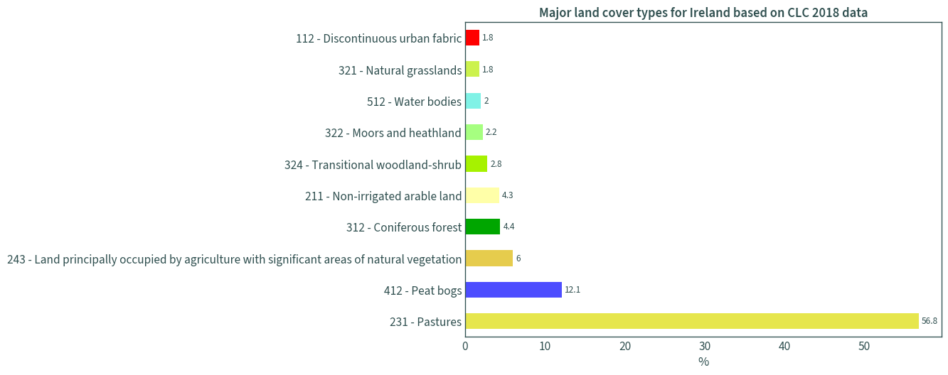
| 0 | 18 | 4779044.0 | #e6e64d | 231 - Pastures | 56.8 |
| 1 | 36 | 1021610.0 | #4d4dff | 412 - Peat bogs | 12.1 |
| 2 | 21 | 508503.0 | #e6cc4d | 243 - Land principally occupied by agriculture... | 6.0 |
| 3 | 24 | 371866.0 | #00a600 | 312 - Coniferous forest | 4.4 |
| 4 | 12 | 360712.0 | #ffffa8 | 211 - Non-irrigated arable land | 4.3 |
| 5 | 29 | 239577.0 | #a6f200 | 324 - Transitional woodland-shrub | 2.8 |
| 6 | 27 | 188930.0 | #a6ff80 | 322 - Moors and heathland | 2.2 |
| 7 | 41 | 169123.0 | #80f2e6 | 512 - Water bodies | 2.0 |
| 8 | 26 | 150786.0 | #ccf24d | 321 - Natural grasslands | 1.8 |
| 9 | 2 | 148763.0 | #ff0000 | 112 - Discontinuous urban fabric | 1.8 |
| 10 | 25 | 80859.0 | #4dff00 | 313 - Mixed forest | 1.0 |
| 11 | 20 | 80572.0 | #ffe64d | 242 - Complex cultivation patterns | 1.0 |
| 12 | 23 | 61106.0 | #80ff00 | 311 - Broad-leaved forest | 0.7 |
| 13 | 32 | 55614.0 | #ccffcc | 333 - Sparsely vegetated areas | 0.7 |
| 14 | 11 | 29636.0 | #ffe6ff | 142 - Sport and leisure facilities | 0.4 |
| 15 | 35 | 24772.0 | #a6a6ff | 411 - Inland marshes | 0.3 |
| 16 | 3 | 22842.0 | #cc4df2 | 121 - Industrial or commercial units | 0.3 |
| 17 | 31 | 18999.0 | #cccccc | 332 - Bare rocks | 0.2 |
| 18 | 7 | 12726.0 | #a600cc | 131 - Mineral extraction sites | 0.2 |
| 19 | 44 | 12274.0 | #e6f2ff | 523 - Sea and ocean | 0.1 |
| 20 | 30 | 9381.0 | #e6e6e6 | 331 - Beaches - dunes - sands | 0.1 |
| 21 | 39 | 8828.0 | #a6a6e6 | 423 - Intertidal flats | 0.1 |
| 22 | 40 | 8576.0 | #00ccf2 | 511 - Water courses | 0.1 |
| 23 | 33 | 7918.0 | #000000 | 334 - Burnt areas | 0.1 |
| 24 | 4 | 7132.0 | #cc0000 | 122 - Road and rail networks and associated land | 0.1 |
| 25 | 1 | 6734.0 | #e6004d | 111 - Continuous urban fabric | 0.1 |
| 26 | 43 | 5840.0 | #a6ffe6 | 522 - Estuaries | 0.1 |
| 27 | 10 | 4019.0 | #ffa6ff | 141 - Green urban areas | 0.0 |
| 28 | 6 | 3946.0 | #e6cce6 | 124 - Airports | 0.0 |
| 29 | 37 | 3773.0 | #ccccff | 421 - Salt marshes | 0.0 |
| 30 | 9 | 1428.0 | #ff4dff | 133 - Construction sites | 0.0 |
| 31 | 8 | 1329.0 | #a64d00 | 132 - Dump sites | 0.0 |
| 32 | 5 | 1183.0 | #e6cccc | 123 - Port areas | 0.0 |
| 33 | 42 | 970.0 | #00ffa6 | 521 - Coastal lagoons | 0.0 |
| 34 | 16 | 372.0 | #f2a64d | 222 - Fruit trees and berry plantations | 0.0 |
# plot major land cover types, i.e. percentage > 1
mask = uniquevals["percentage"] > 1
uniquevals_sig = uniquevals[mask]
ax = uniquevals_sig.plot.barh(
x="label",
y="percentage",
legend=False,
figsize=(9, 6),
color=uniquevals_sig["color"],
)
ax.bar_label(ax.containers[0], padding=3)
plt.title("Major land cover types for Ireland based on CLC 2018 data")
plt.ylabel("")
plt.xlabel("%")
plt.show()
# convert values to integer and sort
uniquevals["value"] = uniquevals["value"].astype(int)
uniquevals.sort_values("value", inplace=True)
# create a colourmap for the plot
colours = list(uniquevals["color"])
nodes = np.array(uniquevals["value"])
# normalisation
nodes = (nodes - min(nodes)) / (max(nodes) - min(nodes))
colours = LinearSegmentedColormap.from_list(
"CLC2018", list(zip(nodes, colours))
)
colours
CLC2018

under
bad
over
col_discrete = ListedColormap(list(uniquevals["color"]))
col_discrete
from_list

under
bad
over
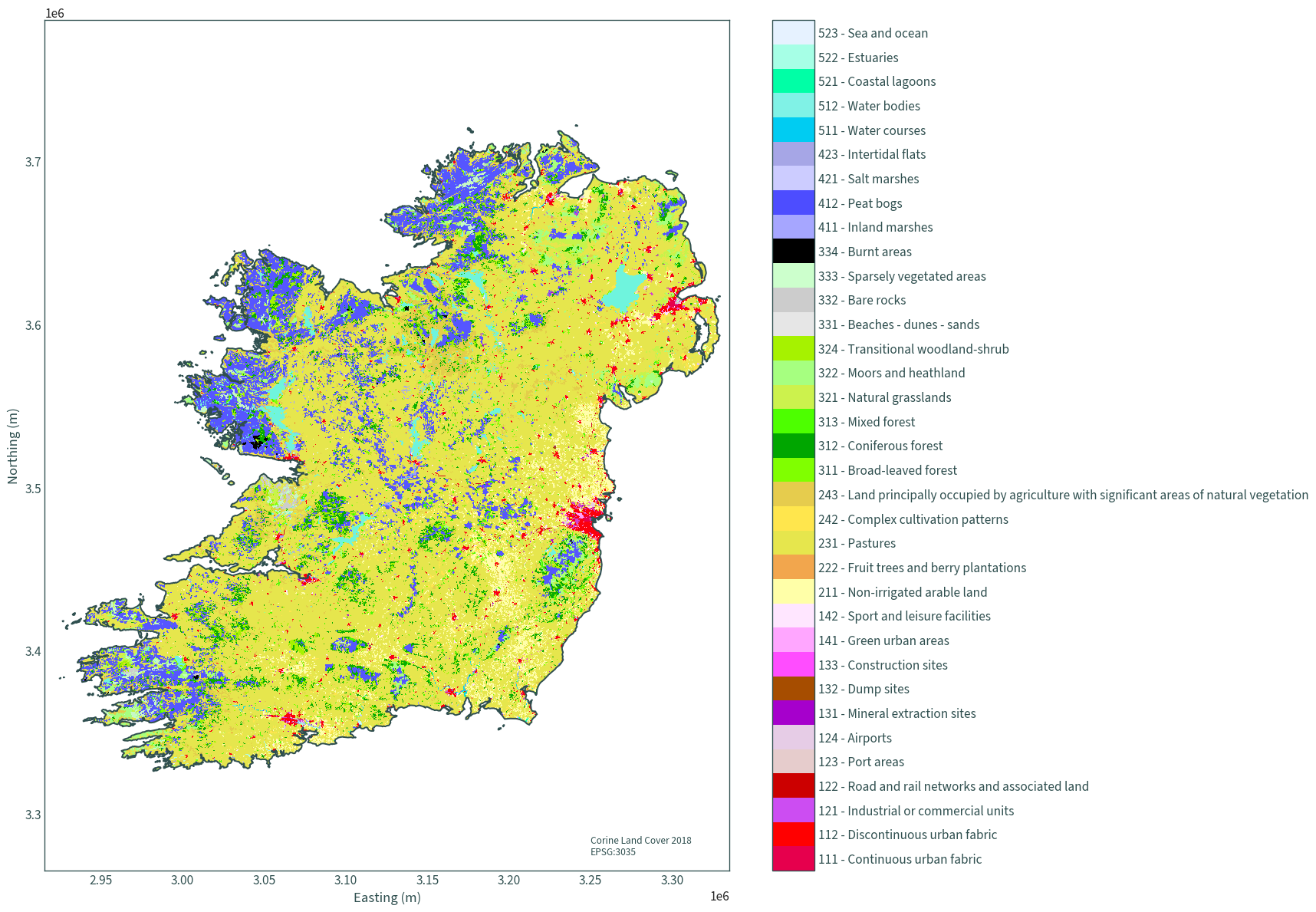
img = plt.figure(figsize=(15, 15))
img = plt.imshow(np.array([[0, len(uniquevals)]]), cmap=col_discrete)
img.set_visible(False)
ticks = list(np.arange(0.5, len(uniquevals) + 0.5, 1))
cbar = plt.colorbar(ticks=ticks)
cbar.ax.set_yticklabels(list(uniquevals["label"]))
landcover.plot(add_colorbar=False, cmap=colours)
ie.boundary.plot(ax=img.axes, color="darkslategrey")
# plt.title("CLC 2018 - Ireland")
plt.title(None)
plt.xlabel("Easting (m)")
plt.ylabel("Northing (m)")
plt.axis("equal")
plt.text(3.25e6, 3.275e6, "Corine Land Cover 2018\nEPSG:3035")
plt.xlim(landcover.rio.bounds()[0] - 9e3, landcover.rio.bounds()[1] + 9e3)
plt.ylim(landcover.rio.bounds()[2] - 9e3, landcover.rio.bounds()[3] + 9e3)
plt.show()
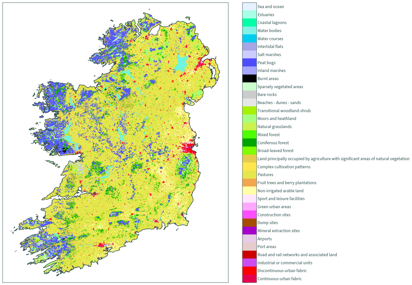
uniquevals["label"] = uniquevals["label"].str[6:]
img = plt.figure(figsize=(15, 15))
img = plt.imshow(np.array([[0, len(uniquevals)]]), cmap=col_discrete)
img.set_visible(False)
ticks = list(np.arange(0.5, len(uniquevals) + 0.5, 1))
cbar = plt.colorbar(ticks=ticks)
cbar.ax.set_yticklabels(list(uniquevals["label"]))
landcover.rio.reproject(cplt.projection_hiresireland).plot(
add_colorbar=False, cmap=colours
)
ie.to_crs(cplt.projection_hiresireland).boundary.plot(
ax=img.axes, edgecolor="darkslategrey"
)
plt.title(None)
img.axes.tick_params(labelbottom=False, labelleft=False)
plt.xlabel("")
plt.ylabel("")
plt.axis("equal")
bbox = ie.to_crs(cplt.projection_hiresireland).bounds
plt.xlim(float(bbox["minx"]) - 0.1, float(bbox["maxx"]) + 0.1)
plt.ylim(float(bbox["miny"]) - 0.1, float(bbox["maxy"]) + 0.1)
plt.show()
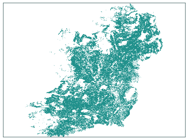
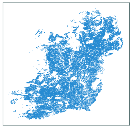
# pastures
lc = landcover.where(landcover.compute() == 18, drop=True)
lc
<xarray.DataArray (band: 1, y: 3911, x: 3988)>
array([[[nan, nan, nan, ..., nan, nan, nan],
        [nan, nan, nan, ..., nan, nan, nan],
        [nan, nan, nan, ..., nan, nan, nan],
        ...,
        [nan, nan, nan, ..., nan, nan, nan],
        [nan, nan, nan, ..., nan, nan, nan],
        [nan, nan, nan, ..., nan, nan, nan]]])
Coordinates:
* x (x) float64 2.928e+06 2.928e+06 ... 3.329e+06 3.329e+06
* y (y) float64 3.719e+06 3.718e+06 ... 3.328e+06 3.328e+06
* band (band) int64 1
spatial_ref int64 0
Attributes:
AREA_OR_POINT: Area
DataType: Thematic
RepresentationType: THEMATIC
STATISTICS_COVARIANCES: 136.429646247598
STATISTICS_MAXIMUM: 48
STATISTICS_MEAN: 25.753373398066
STATISTICS_MINIMUM: 1
STATISTICS_SKIPFACTORX: 1
STATISTICS_SKIPFACTORY: 1
STATISTICS_STDDEV: 11.680310194836
scale_factor: 1.0
add_offset: 0.0fig = lc.plot(add_colorbar=False)
fig.axes.tick_params(labelbottom=False, labelleft=False)
plt.title(None)
plt.axis("equal")
plt.xlabel("")
plt.ylabel("")
plt.tight_layout()
plt.show()
# export to GeoTIFF
lc.rio.to_raster(
os.path.join(DATA_DIR_BASE, "clc-2018-ie-pasture.tif"),
windowed=True,
tiled=True,
)
lc
<xarray.DataArray (band: 1, y: 3911, x: 3988)>
array([[[nan, nan, nan, ..., nan, nan, nan],
        [nan, nan, nan, ..., nan, nan, nan],
        [nan, nan, nan, ..., nan, nan, nan],
        ...,
        [nan, nan, nan, ..., nan, nan, nan],
        [nan, nan, nan, ..., nan, nan, nan],
        [nan, nan, nan, ..., nan, nan, nan]]])
Coordinates:
  * x            (x) float64 2.928e+06 2.928e+06 ... 3.329e+06 3.329e+06
  * y            (y) float64 3.719e+06 3.718e+06 ... 3.328e+06 3.328e+06
  * band         (band) int64 1
    spatial_ref  int64 0
Attributes:
    AREA_OR_POINT:           Area
    DataType:                Thematic
    RepresentationType:      THEMATIC
    STATISTICS_COVARIANCES:  136.429646247598
    STATISTICS_MAXIMUM:      48
    STATISTICS_MEAN:         25.753373398066
    STATISTICS_MINIMUM:      1
    STATISTICS_SKIPFACTORX:  1
    STATISTICS_SKIPFACTORY:  1
    STATISTICS_STDDEV:       11.680310194836
    scale_factor:            1.0
add_offset: 0.0# vectorised
pasture = lc.to_dataframe(name="lc").reset_index().dropna()
pasture = gpd.GeoDataFrame(
    geometry=gpd.GeoSeries(gpd.points_from_xy(pasture.x, pasture.y))
    .buffer(50)
    .envelope,
    crs=lc.rio.crs,
).dissolve()
fig = pasture.plot()
fig.axes.tick_params(labelbottom=False, labelleft=False)
plt.tight_layout()
plt.show()
pasture.to_file(
    os.path.join(DATA_DIR_BASE, "clc-2018-pasture.gpkg"), layer="dissolved"
)