Grass growth anomalies - seasonal#
Weighted means take into account the number of days in each month
import glob
import itertools
import os
import sys
from datetime import datetime, timezone
import geopandas as gpd
import matplotlib.pyplot as plt
import numpy as np
import xarray as xr
import climag.climag as cplt
from climag import climag_plot
exp_list = ["historical", "rcp45", "rcp85"]
model_list = ["CNRM-CM5", "EC-EARTH", "HadGEM2-ES", "MPI-ESM-LR"]
dataset_list = ["EURO-CORDEX", "HiResIreland"]
def keep_minimal_vars(data):
    """
    Drop variables that are not needed
    """

    data = data.drop_vars(
        [
            "bm_gv",
            "bm_gr",
            "bm_dv",
            "bm_dr",
            "age_gv",
            "age_gr",
            "age_dv",
            "age_dr",
            "omd_gv",
            "omd_gr",
            "lai",
            "env",
            "wr",
            "aet",
            "sen_gv",
            "sen_gr",
            "abs_dv",
            "abs_dr",
            "i_bm",
            "h_bm",
            "pgro",
            "c_bm",  # "bm"
        ]
    )

    return data
def combine_datasets(dataset_dict, dataset_crs):
    dataset = xr.combine_by_coords(
        dataset_dict.values(), combine_attrs="override"
    )
    dataset.rio.write_crs(dataset_crs, inplace=True)

    return dataset
def mean_wgt(ds, months):
    ds_m = ds.sel(time=ds["time"].dt.month.isin(months))

    weights = (
        ds_m["time"].dt.days_in_month.groupby("time.year")
        / ds_m["time"].dt.days_in_month.groupby("time.year").sum()
    )

    # test that the sum of weights for each season is one
    np.testing.assert_allclose(
        weights.groupby("time.year").sum().values,
        np.ones(len(set(weights["year"].values))),
    )

    # calculate the weighted average
    ds_m = (ds_m * weights).groupby("time.year").sum(dim="time")

    return ds_m
def reduce_dataset(dataset):
    ds = {}
    ds_son = {}
    ds_mam = {}
    ds_jja = {}

    for exp, model in itertools.product(exp_list, model_list):
        # auto-rechunking may cause NotImplementedError with object dtype
        # where it will not be able to estimate the size in bytes of object
        # data
        if model == "HadGEM2-ES":
            CHUNKS = 300
        else:
            CHUNKS = "auto"

        ds[f"{model}_{exp}"] = xr.open_mfdataset(
            glob.glob(
                os.path.join(
                    "data",
                    "ModVege",
                    dataset,
                    exp,
                    model,
                    f"*{dataset}*{model}*{exp}*.nc",
                )
            ),
            chunks=CHUNKS,
            decode_coords="all",
        )

        # copy CRS
        crs_ds = ds[f"{model}_{exp}"].rio.crs

        # remove spin-up year
        if exp == "historical":
            ds[f"{model}_{exp}"] = ds[f"{model}_{exp}"].sel(
                time=slice("1976", "2005")
            )
        else:
            ds[f"{model}_{exp}"] = ds[f"{model}_{exp}"].sel(
                time=slice("2041", "2070")
            )

        # convert HadGEM2-ES data back to 360-day calendar
        # this ensures that the correct weighting is applied when
        # calculating the weighted average
        if model == "HadGEM2-ES":
            ds[f"{model}_{exp}"] = ds[f"{model}_{exp}"].convert_calendar(
                "360_day", align_on="year"
            )

        # assign new coordinates and dimensions
        ds[f"{model}_{exp}"] = ds[f"{model}_{exp}"].assign_coords(exp=exp)
        ds[f"{model}_{exp}"] = ds[f"{model}_{exp}"].expand_dims(dim="exp")
        ds[f"{model}_{exp}"] = ds[f"{model}_{exp}"].assign_coords(model=model)
        ds[f"{model}_{exp}"] = ds[f"{model}_{exp}"].expand_dims(dim="model")

        # calculate cumulative biomass
        ds[f"{model}_{exp}"] = ds[f"{model}_{exp}"].assign(
            bm_t=(
                ds[f"{model}_{exp}"]["bm"]
                + ds[f"{model}_{exp}"]["i_bm"]
                + ds[f"{model}_{exp}"]["h_bm"]
            )
        )

        # drop unnecessary variables
        ds[f"{model}_{exp}"] = keep_minimal_vars(data=ds[f"{model}_{exp}"])

        # weighted mean - yearly, SON
        ds_son[f"{model}_{exp}"] = mean_wgt(ds[f"{model}_{exp}"], [9, 10, 11])

        # weighted mean - yearly, MAM
        ds_mam[f"{model}_{exp}"] = mean_wgt(ds[f"{model}_{exp}"], [3, 4, 5])

        # weighted mean - yearly, JJA
        ds_jja[f"{model}_{exp}"] = mean_wgt(ds[f"{model}_{exp}"], [6, 7, 8])

    # combine data
    # ds = combine_datasets(ds, crs_ds)
    ds_son = combine_datasets(ds_son, crs_ds)
    ds_mam = combine_datasets(ds_mam, crs_ds)
    ds_jja = combine_datasets(ds_jja, crs_ds)

    # ensemble mean
    ds_son = ds_son.mean(dim="model", skipna=True)
    ds_mam = ds_mam.mean(dim="model", skipna=True)
    ds_jja = ds_jja.mean(dim="model", skipna=True)

    # long-term average
    ds_son_lta = ds_son.mean(dim="year", skipna=True)
    ds_mam_lta = ds_mam.mean(dim="year", skipna=True)
    ds_jja_lta = ds_jja.mean(dim="year", skipna=True)

    return ds_son, ds_son_lta, ds_jja, ds_jja_lta, ds_mam, ds_mam_lta
def plot_diff(data, levels, mask=True, plot_var="gro", cmap="BrBG"):
    for exp in list(data["exp"].values):
        print(exp)
        if exp == "historical":
            data_plot = data.sel(year=slice("1976", "2005"))
        else:
            data_plot = data.sel(year=slice("2041", "2070"))
        fig = data_plot.sel(exp=exp)[plot_var].plot.contourf(
            x="rlon",
            y="rlat",
            col="year",
            col_wrap=6,
            subplot_kws={"projection": cplt.projection_hiresireland},
            transform=cplt.rotated_pole_transform(data),
            xlim=(-1.775, 1.6),
            ylim=(-2.1, 2.1),
            figsize=(12, 15.25),
            extend="both",
            robust=True,
            cmap="BrBG",
            levels=climag_plot.colorbar_levels(levels),
            cbar_kwargs={
                "label": "kg DM ha⁻¹ day⁻¹",
                "aspect": 40,
                "location": "bottom",
                "fraction": 0.085,
                "shrink": 0.85,
                "pad": 0.025,
                "extendfrac": "auto",
                "ticks": climag_plot.colorbar_ticks(levels),
            },
        )
        for axis in fig.axs.flat:
            if mask:
                mask_layer.to_crs(cplt.projection_hiresireland).plot(
                    ax=axis, color="white", linewidth=0
                )
            ie_bbox.to_crs(cplt.projection_hiresireland).plot(
                ax=axis,
                edgecolor="darkslategrey",
                color="white",
                linewidth=0.5,
            )
        fig.set_titles("{value}", weight="semibold", fontsize=14)
        plt.show()
# mask out non-pasture areas
mask_layer = gpd.read_file(
    os.path.join("data", "boundaries", "boundaries_all.gpkg"),
    layer="CLC_2018_MASK_PASTURE_2157_IE",
)
# mask for offshore areas
ie_bbox = gpd.read_file(
    os.path.join("data", "boundaries", "boundaries_all.gpkg"),
    layer="ne_10m_land_2157_IE_BBOX_DIFF",
)
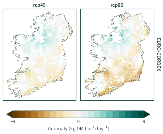
EURO-CORDEX#
ds_son, ds_son_lta, ds_jja, ds_jja_lta, ds_mam, ds_mam_lta = reduce_dataset(
    "EURO-CORDEX"
)
Anomalies in SON growth compared to the historical LTA#
plot_data = (
    (
        ds_son.mean(dim="year", skipna=True)
        - ds_son_lta.sel(exp="historical").drop_vars("exp")
    )
    .sel(exp=["rcp45", "rcp85"])
    .assign_coords(dataset="EURO-CORDEX")
    .expand_dims(dim="dataset")
)
fig = plot_data["gro"].plot.contourf(
    x="rlon",
    y="rlat",
    col="exp",
    row="dataset",
    robust=True,
    extend="both",
    cmap="BrBG",
    subplot_kws={"projection": cplt.projection_hiresireland},
    transform=cplt.rotated_pole_transform(plot_data),
    xlim=(-1.775, 1.6),
    ylim=(-2.1, 2.1),
    figsize=(6, 4.75),
    levels=climag_plot.colorbar_levels(9),
    cbar_kwargs={
        "label": "Anomaly [kg DM ha⁻¹ day⁻¹]",
        "aspect": 20,
        "location": "bottom",
        "fraction": 0.085,
        "shrink": 0.95,
        "pad": 0.085,
        "extendfrac": "auto",
        "ticks": climag_plot.colorbar_ticks(9),
    },
)
for axis in fig.axs.flat:
    mask_layer.to_crs(cplt.projection_hiresireland).plot(
        ax=axis, color="white", linewidth=0
    )
    ie_bbox.to_crs(cplt.projection_hiresireland).plot(
        ax=axis, edgecolor="darkslategrey", color="white", linewidth=0.5
    )
fig.set_titles("{value}", weight="semibold", fontsize=14)
plt.show()
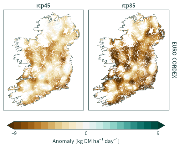
Summer#
plot_data = (
    (
        ds_jja.mean(dim="year", skipna=True)
        - ds_jja_lta.sel(exp="historical").drop_vars("exp")
    )
    .sel(exp=["rcp45", "rcp85"])
    .assign_coords(dataset="EURO-CORDEX")
    .expand_dims(dim="dataset")
)

fig = plot_data["gro"].plot.contourf(
    x="rlon",
    y="rlat",
    col="exp",
    row="dataset",
    robust=True,
    extend="both",
    cmap="BrBG",
    subplot_kws={"projection": cplt.projection_hiresireland},
    transform=cplt.rotated_pole_transform(plot_data),
    xlim=(-1.775, 1.6),
    ylim=(-2.1, 2.1),
    figsize=(6, 4.75),
    levels=climag_plot.colorbar_levels(9),
    cbar_kwargs={
        "label": "Anomaly [kg DM ha⁻¹ day⁻¹]",
        "aspect": 20,
        "location": "bottom",
        "fraction": 0.085,
        "shrink": 0.95,
        "pad": 0.085,
        "extendfrac": "auto",
        "ticks": climag_plot.colorbar_ticks(9),
    },
)
for axis in fig.axs.flat:
    mask_layer.to_crs(cplt.projection_hiresireland).plot(
        ax=axis, color="white", linewidth=0
    )
    ie_bbox.to_crs(cplt.projection_hiresireland).plot(
        ax=axis, edgecolor="darkslategrey", color="white", linewidth=0.5
    )
fig.set_titles("{value}", weight="semibold", fontsize=14)
plt.show()
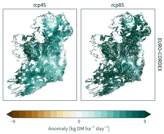
Spring#
plot_data = (
    (
        ds_mam.mean(dim="year", skipna=True)
        - ds_mam_lta.sel(exp="historical").drop_vars("exp")
    )
    .sel(exp=["rcp45", "rcp85"])
    .assign_coords(dataset="EURO-CORDEX")
    .expand_dims(dim="dataset")
)

fig = plot_data["gro"].plot.contourf(
    x="rlon",
    y="rlat",
    col="exp",
    row="dataset",
    robust=True,
    extend="both",
    cmap="BrBG",
    subplot_kws={"projection": cplt.projection_hiresireland},
    transform=cplt.rotated_pole_transform(plot_data),
    xlim=(-1.775, 1.6),
    ylim=(-2.1, 2.1),
    figsize=(6, 4.75),
    levels=climag_plot.colorbar_levels(9),
    cbar_kwargs={
        "label": "Anomaly [kg DM ha⁻¹ day⁻¹]",
        "aspect": 20,
        "location": "bottom",
        "fraction": 0.085,
        "shrink": 0.95,
        "pad": 0.085,
        "extendfrac": "auto",
        "ticks": climag_plot.colorbar_ticks(9),
    },
)
for axis in fig.axs.flat:
    mask_layer.to_crs(cplt.projection_hiresireland).plot(
        ax=axis, color="white", linewidth=0
    )
    ie_bbox.to_crs(cplt.projection_hiresireland).plot(
        ax=axis, edgecolor="darkslategrey", color="white", linewidth=0.5
    )
fig.set_titles("{value}", weight="semibold", fontsize=14)
plt.show()
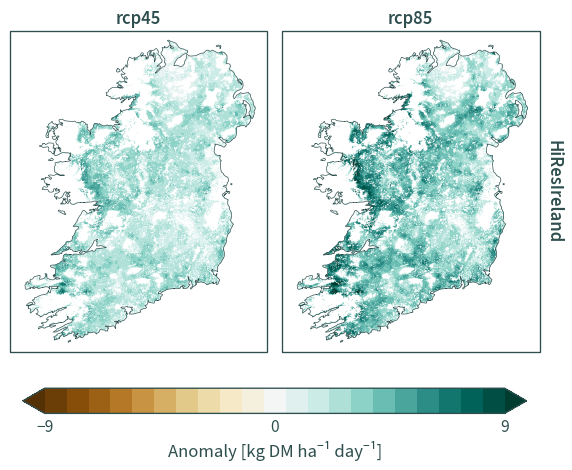
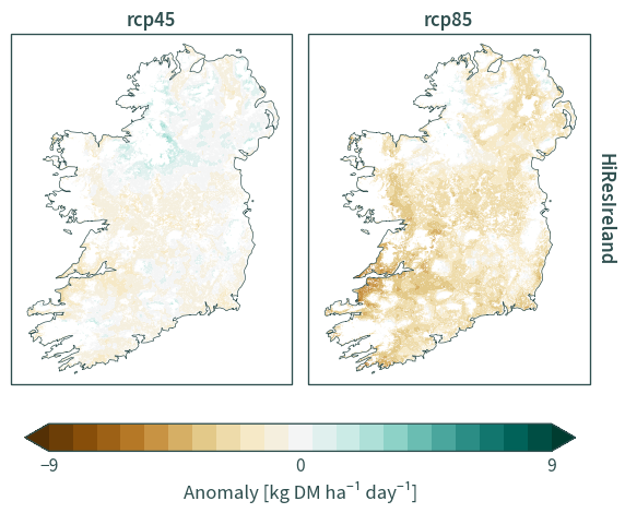
HiResIreland#
ds_son, ds_son_lta, ds_jja, ds_jja_lta, ds_mam, ds_mam_lta = reduce_dataset(
    "HiResIreland"
)
Anomalies in SON growth compared to historical LTA#
plot_data = (
    (
        ds_son.mean(dim="year", skipna=True)
        - ds_son_lta.sel(exp="historical").drop_vars("exp")
    )
    .sel(exp=["rcp45", "rcp85"])
    .assign_coords(dataset="HiResIreland")
    .expand_dims(dim="dataset")
)
fig = plot_data["gro"].plot.contourf(
    x="rlon",
    y="rlat",
    col="exp",
    row="dataset",
    robust=True,
    extend="both",
    cmap="BrBG",
    subplot_kws={"projection": cplt.projection_hiresireland},
    transform=cplt.rotated_pole_transform(plot_data),
    xlim=(-1.775, 1.6),
    ylim=(-2.1, 2.1),
    figsize=(6, 4.75),
    levels=climag_plot.colorbar_levels(9),
    cbar_kwargs={
        "label": "Anomaly [kg DM ha⁻¹ day⁻¹]",
        "aspect": 20,
        "location": "bottom",
        "fraction": 0.085,
        "shrink": 0.95,
        "pad": 0.085,
        "extendfrac": "auto",
        "ticks": climag_plot.colorbar_ticks(9),
    },
)
for axis in fig.axs.flat:
    mask_layer.to_crs(cplt.projection_hiresireland).plot(
        ax=axis, color="white", linewidth=0
    )
    ie_bbox.to_crs(cplt.projection_hiresireland).plot(
        ax=axis, edgecolor="darkslategrey", color="white", linewidth=0.5
    )
fig.set_titles("{value}", weight="semibold", fontsize=14)
plt.show()
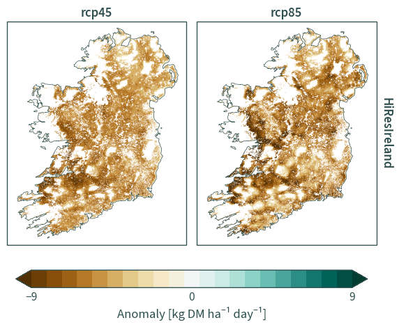
Summer#
plot_data = (
    (
        ds_jja.mean(dim="year", skipna=True)
        - ds_jja_lta.sel(exp="historical").drop_vars("exp")
    )
    .sel(exp=["rcp45", "rcp85"])
    .assign_coords(dataset="HiResIreland")
    .expand_dims(dim="dataset")
)

fig = plot_data["gro"].plot.contourf(
    x="rlon",
    y="rlat",
    col="exp",
    row="dataset",
    robust=True,
    extend="both",
    cmap="BrBG",
    subplot_kws={"projection": cplt.projection_hiresireland},
    transform=cplt.rotated_pole_transform(plot_data),
    xlim=(-1.775, 1.6),
    ylim=(-2.1, 2.1),
    figsize=(6, 4.75),
    levels=climag_plot.colorbar_levels(9),
    cbar_kwargs={
        "label": "Anomaly [kg DM ha⁻¹ day⁻¹]",
        "aspect": 20,
        "location": "bottom",
        "fraction": 0.085,
        "shrink": 0.95,
        "pad": 0.085,
        "extendfrac": "auto",
        "ticks": climag_plot.colorbar_ticks(9),
    },
)
for axis in fig.axs.flat:
    mask_layer.to_crs(cplt.projection_hiresireland).plot(
        ax=axis, color="white", linewidth=0
    )
    ie_bbox.to_crs(cplt.projection_hiresireland).plot(
        ax=axis, edgecolor="darkslategrey", color="white", linewidth=0.5
    )
fig.set_titles("{value}", weight="semibold", fontsize=14)
plt.show()
Spring#
plot_data = (
    (
        ds_mam.mean(dim="year", skipna=True)
        - ds_mam_lta.sel(exp="historical").drop_vars("exp")
    )
    .sel(exp=["rcp45", "rcp85"])
    .assign_coords(dataset="HiResIreland")
    .expand_dims(dim="dataset")
)

fig = plot_data["gro"].plot.contourf(
    x="rlon",
    y="rlat",
    col="exp",
    row="dataset",
    robust=True,
    extend="both",
    cmap="BrBG",
    subplot_kws={"projection": cplt.projection_hiresireland},
    transform=cplt.rotated_pole_transform(plot_data),
    xlim=(-1.775, 1.6),
    ylim=(-2.1, 2.1),
    figsize=(6, 4.75),
    levels=climag_plot.colorbar_levels(9),
    cbar_kwargs={
        "label": "Anomaly [kg DM ha⁻¹ day⁻¹]",
        "aspect": 20,
        "location": "bottom",
        "fraction": 0.085,
        "shrink": 0.95,
        "pad": 0.085,
        "extendfrac": "auto",
        "ticks": climag_plot.colorbar_ticks(9),
    },
)
for axis in fig.axs.flat:
    mask_layer.to_crs(cplt.projection_hiresireland).plot(
        ax=axis, color="white", linewidth=0
    )
    ie_bbox.to_crs(cplt.projection_hiresireland).plot(
        ax=axis, edgecolor="darkslategrey", color="white", linewidth=0.5
    )
fig.set_titles("{value}", weight="semibold", fontsize=14)
plt.show()