Met Éireann Reanalysis (MÉRA) - using GRIB files#
https://www.met.ie/climate/available-data/mera
Issues:
data uses 0/360 longitude coordinates instead of -180/180
data spans both negative and positive longitudes
projection information is not parsed when the data is read
lon/lat are multidimensional coordinates (y, x)
data with two-dimensional coordinates cannot be spatially selected (e.g. extracting data for a certain point, or clipping with a geometry)
x and y correspond to the index of the cells and are not coordinates in Lambert Conformal Conic projection
Solution:
use CDO to convert the GRIB file to netCDF first
projection info is parsed and can be read by Xarray
one-dimensional coordinates in Lambert Conformal Conic projection
data can now be indexed or selected both spatially and temporally using Xarray
some metadata are lost (e.g. variable name and attributes) but these can be reassigned manually
this method combines all three time steps in the example data (data needs to be split prior to conversion to avoid this)
Relevant links:
https://docs.xarray.dev/en/stable/examples/multidimensional-coords.html
https://docs.xarray.dev/en/stable/examples/ERA5-GRIB-example.html
https://scitools.org.uk/cartopy/docs/latest/reference/projections.html
https://confluence.ecmwf.int/display/OIFS/How+to+convert+GRIB+to+netCDF
Example data used: https://www.met.ie/downloads/MERA_PRODYEAR_2015_06_11_105_2_0_FC3hr.grb
Requirements:
CDO
Python 3.10
rioxarray
geopandas
dask
cartopy
matplotlib
nc-time-axis
pooch
netcdf4
cfgrib
import os
from datetime import date, datetime, timezone
import cartopy.crs as ccrs
import geopandas as gpd
import matplotlib.dates as mdates
import matplotlib.pyplot as plt
import matplotlib.units as munits
import numpy as np
import pooch
import xarray as xr
# Moorepark, Fermoy met station coords
LON, LAT = -8.26389, 52.16389
# Ireland boundary (derived from NUTS 2021)
GPKG_BOUNDARY = os.path.join("data", "boundaries", "boundaries_all.gpkg")
ie = gpd.read_file(GPKG_BOUNDARY, layer="NUTS_RG_01M_2021_2157_IE")
DATA_DIR = os.path.join("data", "MERA", "sample")
os.makedirs(DATA_DIR, exist_ok=True)
URL = "https://www.met.ie/downloads/MERA_PRODYEAR_2015_06_11_105_2_0_FC3hr.grb"
FILE_NAME = "MERA_PRODYEAR_2015_06_11_105_2_0_FC3hr"
# download data if necessary
# sample GRIB data; 2 m temperature; 3-h forecasts
if not os.path.isfile(os.path.join(DATA_DIR, FILE_NAME)):
    pooch.retrieve(
        url=URL, known_hash=None, fname=f"{FILE_NAME}.grb", path=DATA_DIR
    )

    with open(
        os.path.join(DATA_DIR, f"{FILE_NAME}.txt"), "w", encoding="utf-8"
    ) as outfile:
        outfile.write(
            f"Data downloaded on: {datetime.now(tz=timezone.utc)}\n"
            f"Download URL: {URL}"
        )
# path to example data file
BASE_FILE_NAME = os.path.join(DATA_DIR, FILE_NAME)
Read original GRIB data#
data = xr.open_dataset(
    f"{BASE_FILE_NAME}.grb",
    decode_coords="all",
    chunks="auto",
    engine="cfgrib",
)
data
<xarray.Dataset>
Dimensions:            (time: 240, step: 3, y: 489, x: 529)
Coordinates:
  * time               (time) datetime64[ns] 2015-06-01 ... 2015-06-30T21:00:00
  * step               (step) timedelta64[ns] 01:00:00 02:00:00 03:00:00
    heightAboveGround  float64 ...
    latitude           (y, x) float64 dask.array<chunksize=(489, 529), meta=np.ndarray>
    longitude          (y, x) float64 dask.array<chunksize=(489, 529), meta=np.ndarray>
    valid_time         (time, step) datetime64[ns] dask.array<chunksize=(240, 3), meta=np.ndarray>
Dimensions without coordinates: y, x
Data variables:
    t                  (time, step, y, x) float32 dask.array<chunksize=(194, 1, 398, 432), meta=np.ndarray>
Attributes:
    GRIB_edition:            1
    GRIB_centre:             eidb
    GRIB_centreDescription:  Dublin
    GRIB_subCentre:          255
    Conventions:             CF-1.7
    institution:             Dublin
history: 2023-04-01T21:49 GRIB to CDM+CF via cfgrib-0.9.1...# view CRS
data.rio.crs
# save variable attributes
t_attrs = data["t"].attrs
# convert 0/360 deg to -180/180 deg lon
long_attrs = data.longitude.attrs
data = data.assign_coords(longitude=(((data.longitude + 180) % 360) - 180))
# reassign attributes
data.longitude.attrs = long_attrs
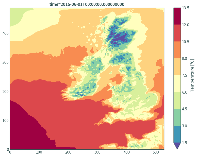
Plots#
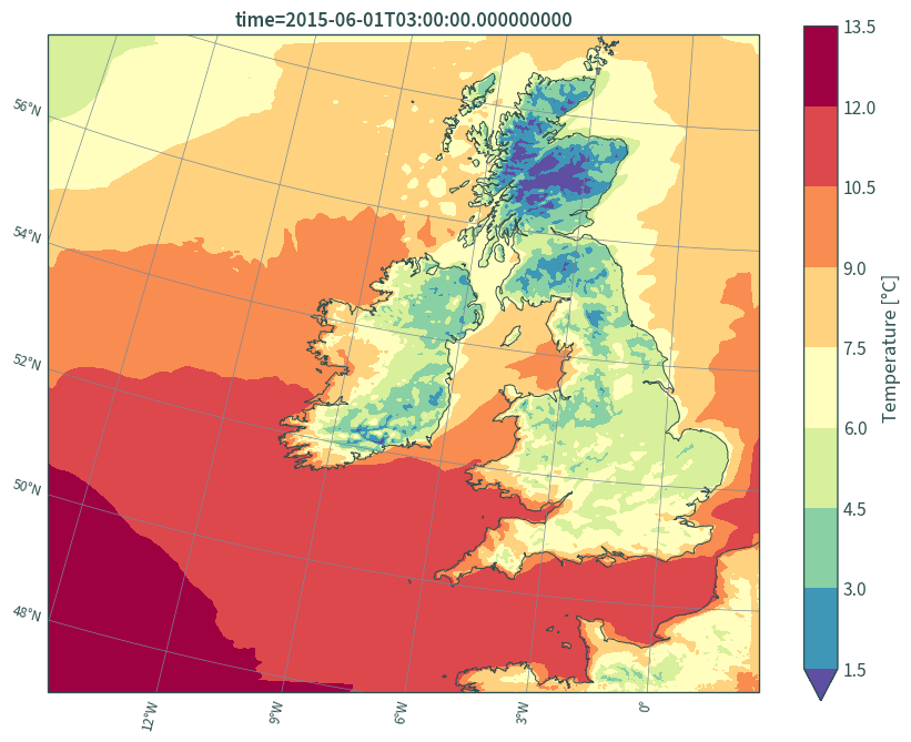
plt.figure(figsize=(9, 7))
(data.isel(time=0, step=2)["t"] - 273.15).plot.contourf(
    robust=True,
    cmap="Spectral_r",
    levels=11,
    cbar_kwargs={"label": "Temperature [°C]"},
)
plt.tight_layout()
plt.xlabel(None)
plt.ylabel(None)
plt.title(f"time={data.isel(time=0, step=2)['t']['time'].values}")
plt.show()
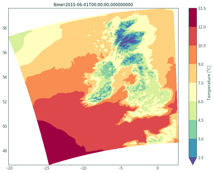
# specifying lon/lat as the x/y axes
plt.figure(figsize=(9, 7))
(data.isel(time=0, step=2)["t"] - 273.15).plot.contourf(
    robust=True,
    cmap="Spectral_r",
    x="longitude",
    y="latitude",
    cbar_kwargs={"label": "Temperature [°C]"},
    levels=11,
)
plt.xlabel(None)
plt.ylabel(None)
plt.title(f"time={data.isel(time=0, step=2)['t']['time'].values}")
plt.tight_layout()
plt.show()
Convert GRIB to netCDF using CDO#
# keep only the third forecast step and convert to netCDF
os.system(
    f"cdo -s -f nc4c -copy -seltimestep,3/{len(data['time']) * 3}/3 "
    f"{BASE_FILE_NAME}.grb {BASE_FILE_NAME}.nc"
)
0
Read data#
data = xr.open_dataset(
    f"{BASE_FILE_NAME}.nc", decode_coords="all", chunks="auto"
)
data
<xarray.Dataset>
Dimensions:            (time: 240, x: 529, y: 489, height: 1)
Coordinates:
  * time               (time) datetime64[ns] 2015-06-01T03:00:00 ... 2015-07-01
  * x                  (x) float64 0.0 2.5e+03 5e+03 ... 1.318e+06 1.32e+06
  * y                  (y) float64 0.0 2.5e+03 5e+03 ... 1.218e+06 1.22e+06
    Lambert_Conformal  int32 ...
  * height             (height) float64 2.0
Data variables:
    var11              (time, height, y, x) float32 dask.array<chunksize=(194, 1, 399, 432), meta=np.ndarray>
Attributes:
    CDI:          Climate Data Interface version 2.0.5 (https://mpimet.mpg.de...
    Conventions:  CF-1.6
    history:      Sat Mar 25 22:55:27 2023: cdo -s -f nc4c -copy -seltimestep...
CDO: Climate Data Operators version 2.0.5 (https://mpimet.mpg.de...data.rio.crs
CRS.from_wkt('PROJCS["undefined",GEOGCS["undefined",DATUM["undefined",SPHEROID["undefined",6367470,0]],PRIMEM["Greenwich",0,AUTHORITY["EPSG","8901"]],UNIT["degree",0.0174532925199433]],PROJECTION["Lambert_Conformal_Conic_1SP"],PARAMETER["latitude_of_origin",53.5],PARAMETER["central_meridian",5],PARAMETER["scale_factor",1],PARAMETER["false_easting",1481641.67696368],PARAMETER["false_northing",537326.063885016],UNIT["metre",1,AUTHORITY["EPSG","9001"]],AXIS["Easting",EAST],AXIS["Northing",NORTH]]')
# reassign attributes and rename variables
data["var11"].attrs = t_attrs
data = data.rename({"var11": "t"})
data
<xarray.Dataset>
Dimensions:            (time: 240, x: 529, y: 489, height: 1)
Coordinates:
  * time               (time) datetime64[ns] 2015-06-01T03:00:00 ... 2015-07-01
  * x                  (x) float64 0.0 2.5e+03 5e+03 ... 1.318e+06 1.32e+06
  * y                  (y) float64 0.0 2.5e+03 5e+03 ... 1.218e+06 1.22e+06
    Lambert_Conformal  int32 ...
  * height             (height) float64 2.0
Data variables:
    t                  (time, height, y, x) float32 dask.array<chunksize=(194, 1, 399, 432), meta=np.ndarray>
Attributes:
    CDI:          Climate Data Interface version 2.0.5 (https://mpimet.mpg.de...
    Conventions:  CF-1.6
    history:      Sat Mar 25 22:55:27 2023: cdo -s -f nc4c -copy -seltimestep...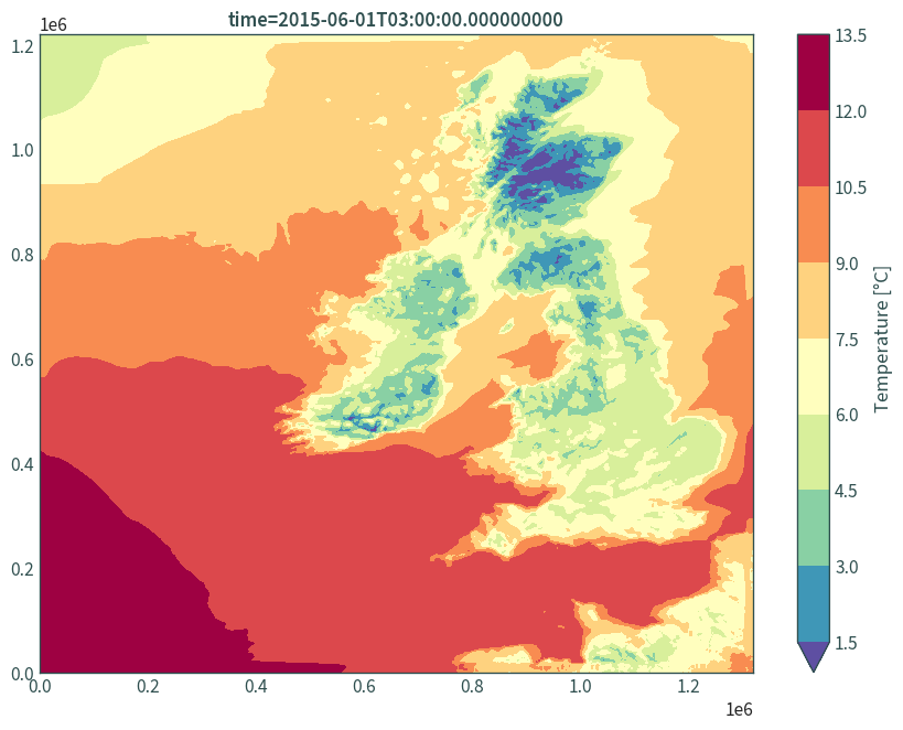
CDO: Climate Data Operators version 2.0.5 (https://mpimet.mpg.de...Plots#
plt.figure(figsize=(9, 7))
(data.isel(time=0, height=0)["t"] - 273.15).plot.contourf(
    robust=True,
    cmap="Spectral_r",
    levels=11,
    cbar_kwargs={"label": "Temperature [°C]"},
)
plt.xlabel(None)
plt.ylabel(None)
plt.title(f"time={data.isel(time=0, height=0)['t']['time'].values}")
plt.tight_layout()
plt.show()
# define Lambert Conformal Conic projection for plots and transformations
# using metadata
lambert_conformal = ccrs.LambertConformal(
    false_easting=data["Lambert_Conformal"].attrs["false_easting"],
    false_northing=data["Lambert_Conformal"].attrs["false_northing"],
    standard_parallels=[data["Lambert_Conformal"].attrs["standard_parallel"]],
    central_longitude=(
        data["Lambert_Conformal"].attrs["longitude_of_central_meridian"]
    ),
    central_latitude=(
        data["Lambert_Conformal"].attrs["latitude_of_projection_origin"]
    ),
)
lambert_conformal
<cartopy.crs.LambertConformal object at 0x7fc44026b100>
plt.figure(figsize=(9, 7))
ax = plt.axes(projection=lambert_conformal)
(data.isel(time=0, height=0)["t"] - 273.15).plot.contourf(
    ax=ax,
    robust=True,
    cmap="Spectral_r",
    x="x",
    y="y",
    levels=11,
    transform=lambert_conformal,
    cbar_kwargs={"label": "Temperature [°C]"},
)
ax.gridlines(
    draw_labels={"bottom": "x", "left": "y"},
    color="lightslategrey",
    linewidth=0.5,
    x_inline=False,
    y_inline=False,
)
ax.coastlines(resolution="10m", color="darkslategrey", linewidth=0.75)
plt.title(f"time={data.isel(time=0, height=0)['t']['time'].values}")
plt.tight_layout()
plt.show()
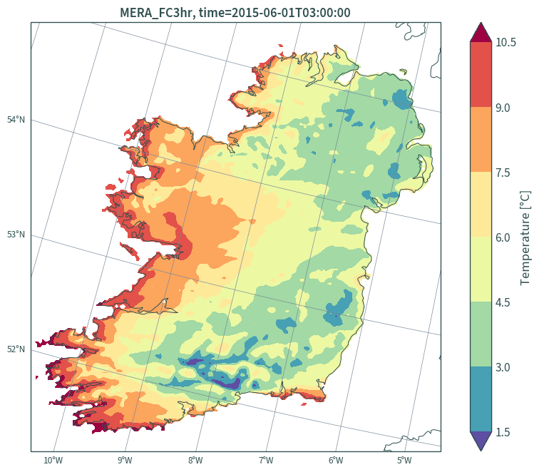
Clip to boundary of Ireland#
data_ie = data.rio.clip(
    ie.buffer(1).to_crs(lambert_conformal), all_touched=True
)
data_ie
<xarray.Dataset>
Dimensions:            (time: 240, x: 158, y: 166, height: 1)
Coordinates:
  * time               (time) datetime64[ns] 2015-06-01T03:00:00 ... 2015-07-01
  * x                  (x) float64 4.15e+05 4.175e+05 ... 8.05e+05 8.075e+05
  * y                  (y) float64 4.075e+05 4.1e+05 ... 8.175e+05 8.2e+05
  * height             (height) float64 2.0
    spatial_ref        int64 0
    Lambert_Conformal  int64 0
Data variables:
    t                  (time, height, y, x) float32 dask.array<chunksize=(194, 1, 166, 158), meta=np.ndarray>
Attributes:
    CDI:          Climate Data Interface version 2.0.5 (https://mpimet.mpg.de...
    Conventions:  CF-1.6
    history:      Sat Mar 25 22:55:27 2023: cdo -s -f nc4c -copy -seltimestep...
CDO: Climate Data Operators version 2.0.5 (https://mpimet.mpg.de...# contour plot
plt.figure(figsize=(9, 7))
ax = plt.axes(projection=ccrs.EuroPP())
(data_ie.isel(time=0, height=0)["t"] - 273.15).plot.contourf(
ax=ax,
robust=True,
cmap="Spectral_r",
x="x",
y="y",
levels=8,
transform=lambert_conformal,
cbar_kwargs={"label": "Temperature [°C]"},
)
ax.gridlines(
draw_labels={"bottom": "x", "left": "y"},
color="lightslategrey",
linewidth=0.5,
x_inline=False,
y_inline=False,
)
ax.coastlines(resolution="10m", color="darkslategrey", linewidth=0.75)
plt.title(
"MERA_FC3hr, "
+ f"time={str(data_ie.isel(time=0, height=0)['t']['time'].values)[:19]}"
)
plt.tight_layout()
plt.show()
# find number of grid cells with data
len(
    data_ie.isel(time=0, height=0)["t"].values.flatten()[
        np.isfinite(data_ie.isel(time=0, height=0)["t"].values.flatten())
    ]
)
14490
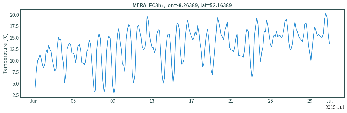
Time series for a point (Moorepark)#
# transform coordinates from lon/lat to Lambert Conformal Conic
XLON, YLAT = lambert_conformal.transform_point(
    x=LON, y=LAT, src_crs=ccrs.PlateCarree()
)
XLON, YLAT
(579021.4574730808, 472854.55040691514)
# extract data for the nearest grid cell to the point
data_ts = data_ie.sel({"x": XLON, "y": YLAT}, method="nearest")
data_ts
<xarray.Dataset>
Dimensions:            (time: 240, height: 1)
Coordinates:
  * time               (time) datetime64[ns] 2015-06-01T03:00:00 ... 2015-07-01
    x                  float64 5.8e+05
    y                  float64 4.725e+05
  * height             (height) float64 2.0
    spatial_ref        int64 0
    Lambert_Conformal  int64 0
Data variables:
    t                  (time, height) float32 dask.array<chunksize=(194, 1), meta=np.ndarray>
Attributes:
    CDI:          Climate Data Interface version 2.0.5 (https://mpimet.mpg.de...
    Conventions:  CF-1.6
    history:      Sat Mar 25 22:55:27 2023: cdo -s -f nc4c -copy -seltimestep...
CDO: Climate Data Operators version 2.0.5 (https://mpimet.mpg.de...converter = mdates.ConciseDateConverter()
munits.registry[np.datetime64] = converter
munits.registry[date] = converter
munits.registry[datetime] = converter
plt.figure(figsize=(12, 4))
plt.plot(data_ts["time"], (data_ts["t"] - 273.15))
plt.ylabel("Temperature [°C]")
plt.title(f"MERA_FC3hr, lon={LON}, lat={LAT}")
plt.tight_layout()
plt.show()