Gridding agricultural census data - MÉRA#
Gridding based on https://james-brennan.github.io/posts/fast_gridding_geopandas/
import os
import itertools
import geopandas as gpd
import matplotlib.pyplot as plt
import numpy as np
import shapely
import xarray as xr
import climag.climag as cplt
Open some gridded climate data#
TS_FILE = os.path.join("data", "MERA", "IE_MERA_FC3hr_3_day.nc")
data = xr.open_dataset(TS_FILE, chunks="auto", decode_coords="all")
data
<xarray.Dataset>
Dimensions:            (x: 158, y: 166, time: 9497)
Coordinates:
  * x                  (x) float64 4.15e+05 4.175e+05 ... 8.05e+05 8.075e+05
  * y                  (y) float64 4.075e+05 4.1e+05 ... 8.175e+05 8.2e+05
    height             float64 ...
    Lambert_Conformal  int64 ...
  * time               (time) datetime64[ns] 1980-01-01 ... 2005-12-31
    spatial_ref        int64 ...
Data variables:
    PAR                (time, y, x) float32 dask.array<chunksize=(4932, 85, 80), meta=np.ndarray>
    PET                (time, y, x) float32 dask.array<chunksize=(4932, 85, 80), meta=np.ndarray>
    T                  (time, y, x) float32 dask.array<chunksize=(4932, 85, 80), meta=np.ndarray>
    PP                 (time, y, x) float32 dask.array<chunksize=(4932, 85, 80), meta=np.ndarray>
Attributes:
    CDI:          Climate Data Interface version 2.0.5 (https://mpimet.mpg.de...
    Conventions:  CF-1.6
    CDO:          Climate Data Operators version 2.0.5 (https://mpimet.mpg.de...
dataset: IE_MERA_FC3hr_3_day# keep only one var
data = data.drop_vars(["PAR", "PET", "PP"])
Use the gridded data’s bounds to generate a gridded vector layer#
data.rio.bounds()
(413750.0, 406250.0, 808750.0, 821250.0)
xmin, ymin, xmax, ymax = data.rio.bounds()
# the difference between two adjacent rotated lat or lon values is the
# cell size
cell_size = float(data["y"][1] - data["y"][0])
# create the cells in a loop
grid_cells = []
for x0 in np.arange(xmin, xmax + cell_size, cell_size):
    for y0 in np.arange(ymin, ymax + cell_size, cell_size):
        # bounds
        x1 = x0 - cell_size
        y1 = y0 + cell_size
        grid_cells.append(shapely.geometry.box(x0, y0, x1, y1))
grid_cells = gpd.GeoDataFrame(
    grid_cells, columns=["geometry"], crs=cplt.projection_lambert_conformal
)
grid_cells.shape
(26553, 1)
grid_cells.head()
| geometry | |
|---|---|
| 0 | POLYGON ((411250.000 406250.000, 411250.000 40... |
| 1 | POLYGON ((411250.000 408750.000, 411250.000 41... |
| 2 | POLYGON ((411250.000 411250.000, 411250.000 41... |
| 3 | POLYGON ((411250.000 413750.000, 411250.000 41... |
| 4 | POLYGON ((411250.000 416250.000, 411250.000 41... |
grid_cells.crs
<cartopy.crs.LambertConformal object at 0x7f63a9f78250>
Subset climate data to visualise the cells#
data_ = data.isel(time=0)
data_
<xarray.Dataset>
Dimensions:            (x: 158, y: 166)
Coordinates:
  * x                  (x) float64 4.15e+05 4.175e+05 ... 8.05e+05 8.075e+05
  * y                  (y) float64 4.075e+05 4.1e+05 ... 8.175e+05 8.2e+05
    height             float64 ...
    Lambert_Conformal  int64 ...
    time               datetime64[ns] 1980-01-01
    spatial_ref        int64 ...
Data variables:
    T                  (y, x) float32 dask.array<chunksize=(85, 80), meta=np.ndarray>
Attributes:
    CDI:          Climate Data Interface version 2.0.5 (https://mpimet.mpg.de...
    Conventions:  CF-1.6
    CDO:          Climate Data Operators version 2.0.5 (https://mpimet.mpg.de...
dataset: IE_MERA_FC3hr_3_day# find number of grid cells with data
len(data_["T"].values.flatten()[np.isfinite(data_["T"].values.flatten())])
14490
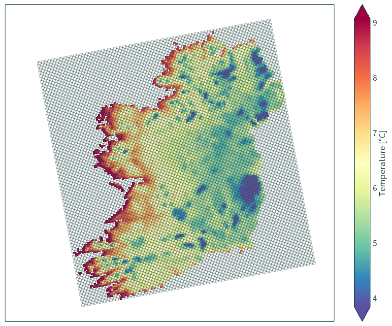
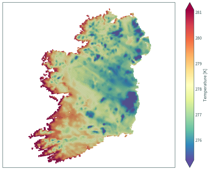
plt.figure(figsize=(9, 7))
axs = plt.axes(projection=cplt.projection_hiresireland)

# plot data for the variable
data_["T"].plot(
    ax=axs,
    cmap="Spectral_r",
    x="x",
    y="y",
    robust=True,
    transform=cplt.projection_lambert_conformal,
)
grid_cells.to_crs(cplt.projection_hiresireland).boundary.plot(
    ax=axs, color="darkslategrey", linewidth=0.2
)

axs.set_title(None)
plt.axis("equal")
plt.tight_layout()
plt.show()
Drop grid cells without climate data#
grid_centroids = {"wkt": [], "x": [], "y": []}

for x, y in itertools.product(
    range(len(data.coords["x"])), range(len(data.coords["y"]))
):
    data__ = data.isel(x=x, y=y)

    # ignore null cells
    if not data__["T"].isnull().all():
        grid_centroids["wkt"].append(
            f"POINT ({float(data__['x'].values)} "
            f"{float(data__['y'].values)})"
        )
        grid_centroids["x"].append(float(data__["x"].values))
        grid_centroids["y"].append(float(data__["y"].values))
grid_centroids = gpd.GeoDataFrame(
    grid_centroids,
    geometry=gpd.GeoSeries.from_wkt(
        grid_centroids["wkt"], crs=cplt.projection_lambert_conformal
    ),
)
grid_centroids.head()
| wkt | x | y | geometry | |
|---|---|---|---|---|
| 0 | POINT (415000.0 497500.0) | 415000.0 | 497500.0 | POINT (415000.000 497500.000) |
| 1 | POINT (417500.0 460000.0) | 417500.0 | 460000.0 | POINT (417500.000 460000.000) |
| 2 | POINT (417500.0 462500.0) | 417500.0 | 462500.0 | POINT (417500.000 462500.000) |
| 3 | POINT (417500.0 492500.0) | 417500.0 | 492500.0 | POINT (417500.000 492500.000) |
| 4 | POINT (417500.0 495000.0) | 417500.0 | 495000.0 | POINT (417500.000 495000.000) |
grid_centroids.shape
(14490, 4)
grid_centroids.crs
<cartopy.crs.LambertConformal object at 0x7fb986ad4310>
grid_cells = gpd.sjoin(
    grid_cells, grid_centroids.to_crs(cplt.projection_lambert_conformal)
)
grid_cells.drop(columns=["wkt", "index_right"], inplace=True)
grid_cells.head()
| geometry | x | y | |
|---|---|---|---|
| 203 | POLYGON ((413750.000 496250.000, 413750.000 49... | 415000.0 | 497500.0 |
| 355 | POLYGON ((416250.000 458750.000, 416250.000 46... | 417500.0 | 460000.0 |
| 356 | POLYGON ((416250.000 461250.000, 416250.000 46... | 417500.0 | 462500.0 |
| 368 | POLYGON ((416250.000 491250.000, 416250.000 49... | 417500.0 | 492500.0 |
| 369 | POLYGON ((416250.000 493750.000, 416250.000 49... | 417500.0 | 495000.0 |
grid_cells.shape
(14490, 3)
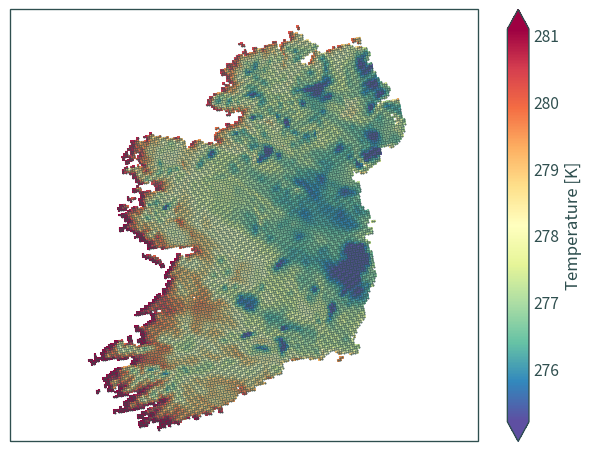
# plt.figure(figsize=(9, 7))
axs = plt.axes(projection=cplt.projection_hiresireland)

# plot data for the variable
data_["T"].plot(
    ax=axs,
    cmap="Spectral_r",
    x="x",
    y="y",
    robust=True,
    transform=cplt.projection_lambert_conformal,
)

grid_cells.to_crs(cplt.projection_hiresireland).plot(
    ax=axs, edgecolor="darkslategrey", facecolor="none", linewidth=0.05
)

grid_centroids.to_crs(cplt.projection_hiresireland).plot(
    ax=axs, color="darkslategrey", markersize=0.2
)

axs.set_title(None)
plt.axis("equal")
plt.tight_layout()
plt.show()
Read stocking rate data#
stocking_rate = gpd.read_file(
    os.path.join("data", "agricultural_census", "agricultural_census.gpkg"),
    layer="stocking_rate",
)
stocking_rate.crs
<Derived Projected CRS: EPSG:2157>
Name: IRENET95 / Irish Transverse Mercator
Axis Info [cartesian]:
- E[east]: Easting (metre)
- N[north]: Northing (metre)
Area of Use:
- name: Ireland - onshore. United Kingdom (UK) - Northern Ireland (Ulster) - onshore.
- bounds: (-10.56, 51.39, -5.34, 55.43)
Coordinate Operation:
- name: Irish Transverse Mercator
- method: Transverse Mercator
Datum: IRENET95
- Ellipsoid: GRS 1980
- Prime Meridian: Greenwich
stocking_rate.head()
| ENGLISH | COUNTY | PROVINCE | GUID | total_cattle | total_sheep | total_grass_hectares | electoral_division | WD22CD | WD22NM | ward_2014_name | stocking_rate | geometry | |
|---|---|---|---|---|---|---|---|---|---|---|---|---|---|
| 0 | TURNAPIN | DUBLIN | Leinster | 2ae19629-1cea-13a3-e055-000000000001 | 0.0 | 0.0 | 0.0 | Turnapin, Co.Dublin, 04042 | 0 | 0 | 0 | 0.000000 | POLYGON ((717716.712 741601.510, 717759.461 74... |
| 1 | DRUMLUMMAN | CAVAN | Ulster | 2ae19629-1caa-13a3-e055-000000000001 | 2673.0 | 231.0 | 1249.1 | Drumlumman, Co.Cavan, 32089 | 0 | 0 | 0 | 1.730446 | POLYGON ((637756.185 787640.988, 637753.646 78... |
| 2 | CASTLEFORE | LEITRIM | Connacht | 2ae19629-171c-13a3-e055-000000000001 | 630.0 | 0.0 | 805.9 | Castlefore, Co.Leitrim, 28063 | 0 | 0 | 0 | 0.625388 | POLYGON ((608196.069 807618.950, 608244.536 80... |
| 3 | RAHONA | CLARE | Munster | 2ae19629-1fec-13a3-e055-000000000001 | 2369.0 | 0.0 | 1349.9 | Rahona, Co.Clare, 16101 | 0 | 0 | 0 | 1.403956 | POLYGON ((484212.068 651795.629, 484231.866 65... |
| 4 | CROSSAKEEL | MEATH | Leinster | 2ae19629-1861-13a3-e055-000000000001 | 4826.0 | 671.0 | 2014.1 | Crossakeel, Co.Meath, 11061 | 0 | 0 | 0 | 1.950201 | POLYGON ((663308.409 776111.796, 663305.294 77... |
stocking_rate.shape
(3917, 13)
stocking_rate["stocking_rate"].max()
5.627624825011666
stocking_rate["stocking_rate"].min()
0.0
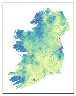
stocking_rate.plot(column="stocking_rate", cmap="Spectral_r")
plt.tick_params(labelbottom=False, labelleft=False)
plt.show()
Reproject cells to the CRS of the stocking rate data#
# use a projected CRS (e.g. 2157) instead of a geographical CRS (e.g. 4326)
grid_cells = grid_cells.to_crs(stocking_rate.crs)
grid_cells.head()
| geometry | x | y | |
|---|---|---|---|
| 203 | POLYGON ((415227.037 594343.036, 414771.907 59... | 415000.0 | 497500.0 |
| 355 | POLYGON ((424513.435 557931.478, 424058.108 56... | 417500.0 | 460000.0 |
| 356 | POLYGON ((424058.108 560389.011, 423602.795 56... | 417500.0 | 462500.0 |
| 368 | POLYGON ((418595.321 589882.162, 418140.190 59... | 417500.0 | 492500.0 |
| 369 | POLYGON ((418140.190 592340.144, 417685.076 59... | 417500.0 | 495000.0 |
axs = stocking_rate.plot(column="stocking_rate", cmap="Spectral_r")
grid_cells.boundary.plot(color="darkslategrey", linewidth=0.2, ax=axs)
axs.tick_params(labelbottom=False, labelleft=False)
plt.show()
Create gridded stocking rate data#
merged = gpd.sjoin(stocking_rate, grid_cells, how="left")
merged.head()
| ENGLISH | COUNTY | PROVINCE | GUID | total_cattle | total_sheep | total_grass_hectares | electoral_division | WD22CD | WD22NM | ward_2014_name | stocking_rate | geometry | index_right | x | y | |
|---|---|---|---|---|---|---|---|---|---|---|---|---|---|---|---|---|
| 0 | TURNAPIN | DUBLIN | Leinster | 2ae19629-1cea-13a3-e055-000000000001 | 0.0 | 0.0 | 0.0 | Turnapin, Co.Dublin, 04042 | 0 | 0 | 0 | 0.000000 | POLYGON ((717716.712 741601.510, 717759.461 74... | 21781 | 737500.0 | 585000.0 |
| 0 | TURNAPIN | DUBLIN | Leinster | 2ae19629-1cea-13a3-e055-000000000001 | 0.0 | 0.0 | 0.0 | Turnapin, Co.Dublin, 04042 | 0 | 0 | 0 | 0.000000 | POLYGON ((717716.712 741601.510, 717759.461 74... | 21782 | 737500.0 | 587500.0 |
| 1 | DRUMLUMMAN | CAVAN | Ulster | 2ae19629-1caa-13a3-e055-000000000001 | 2673.0 | 231.0 | 1249.1 | Drumlumman, Co.Cavan, 32089 | 0 | 0 | 0 | 1.730446 | POLYGON ((637756.185 787640.988, 637753.646 78... | 17129 | 667500.0 | 645000.0 |
| 1 | DRUMLUMMAN | CAVAN | Ulster | 2ae19629-1caa-13a3-e055-000000000001 | 2673.0 | 231.0 | 1249.1 | Drumlumman, Co.Cavan, 32089 | 0 | 0 | 0 | 1.730446 | POLYGON ((637756.185 787640.988, 637753.646 78... | 17296 | 670000.0 | 645000.0 |
| 1 | DRUMLUMMAN | CAVAN | Ulster | 2ae19629-1caa-13a3-e055-000000000001 | 2673.0 | 231.0 | 1249.1 | Drumlumman, Co.Cavan, 32089 | 0 | 0 | 0 | 1.730446 | POLYGON ((637756.185 787640.988, 637753.646 78... | 17130 | 667500.0 | 647500.0 |
merged.shape
(37997, 16)
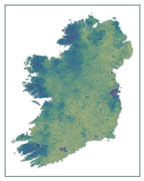
axs = merged.plot(column="stocking_rate", cmap="Spectral_r")
grid_cells.boundary.plot(color="darkslategrey", linewidth=0.2, ax=axs)
axs.tick_params(labelbottom=False, labelleft=False)
plt.show()

# compute stats per grid cell, use the mean stocking rate
dissolve = merged[["stocking_rate", "index_right", "geometry"]].dissolve(
    by="index_right", aggfunc=np.mean
)
dissolve.shape
(14485, 2)
dissolve.head()
| geometry | stocking_rate | |
|---|---|---|
| index_right | ||
| 203 | MULTIPOLYGON (((421214.433 590565.624, 421215.... | 0.917024 |
| 355 | MULTIPOLYGON (((424582.660 560554.883, 424573.... | 0.763591 |
| 356 | MULTIPOLYGON (((424582.660 560554.883, 424573.... | 0.763591 |
| 368 | MULTIPOLYGON (((421214.433 590565.624, 421215.... | 0.917024 |
| 369 | MULTIPOLYGON (((421214.433 590565.624, 421215.... | 0.917024 |
len(dissolve.index.unique())
14485
# merge with cell data
grid_cells.loc[dissolve.index, "sr"] = dissolve["stocking_rate"].values
grid_cells.head()
| geometry | x | y | sr | |
|---|---|---|---|---|
| 203 | POLYGON ((415227.037 594343.036, 414771.907 59... | 415000.0 | 497500.0 | 0.917024 |
| 355 | POLYGON ((424513.435 557931.478, 424058.108 56... | 417500.0 | 460000.0 | 0.763591 |
| 356 | POLYGON ((424058.108 560389.011, 423602.795 56... | 417500.0 | 462500.0 | 0.763591 |
| 368 | POLYGON ((418595.321 589882.162, 418140.190 59... | 417500.0 | 492500.0 | 0.917024 |
| 369 | POLYGON ((418140.190 592340.144, 417685.076 59... | 417500.0 | 495000.0 | 0.917024 |
grid_cells.shape
(14490, 4)
len(grid_cells["geometry"].unique())
14490
grid_cells["sr"].max()
4.190846310810918
grid_cells["sr"].min()
0.0
plt.figure(figsize=(9, 7))
axs = plt.axes(projection=cplt.projection_hiresireland)

# plot data for the variable
data_["t"].plot(
    ax=axs,
    cmap="Spectral_r",
    x="x",
    y="y",
    robust=True,
    transform=cplt.projection_lambert_conformal,
)

grid_cells.to_crs(cplt.projection_hiresireland).plot(
    column="sr",
    ax=axs,
    edgecolor="darkslategrey",
    facecolor="none",
    linewidth=0.2,
)

axs.set_title(None)
plt.axis("equal")
plt.tight_layout()
plt.show()
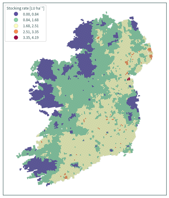
axs = grid_cells.plot(
    column="sr",
    cmap="Spectral_r",
    scheme="equal_interval",
    edgecolor="darkslategrey",
    linewidth=0.2,
    figsize=(6, 7),
    legend=True,
    legend_kwds={
        "loc": "upper left",
        "fmt": "{:.2f}",
        "title": "Stocking rate [LU ha⁻¹]",
    },
)
for legend_handle in axs.get_legend().legend_handles:
    legend_handle.set_markeredgewidth(0.2)
    legend_handle.set_markeredgecolor("darkslategrey")
axs.tick_params(labelbottom=False, labelleft=False)
plt.axis("equal")
plt.tight_layout()
plt.show()
grid_cells.to_file(
    os.path.join("data", "ModVege", "params.gpkg"), layer="mera"
)