Met Éireann Reanalysis - Evapotranspiration#
Derive evapotranspiration using the FAO Penman-Monteith equation
import glob
import os
from datetime import datetime, timezone
import cartopy.crs as ccrs
import matplotlib.pyplot as plt
import numpy as np
import xarray as xr
import climag.climag as cplt
from climag import climag_plot
import seaborn as sns
# directory of processed MÉRA netCDF files
DATA_DIR = os.path.join("/run/media/nms/MyPassport", "MERA", "netcdf_day")
# list of variables needed to derive ET
var_dirs = [
"1_105_0_0", # surface pressure
"15_105_2_2", # max temperature
"16_105_2_2", # min temperature
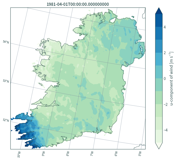
"33_105_10_0", # u-component of 10 m wind
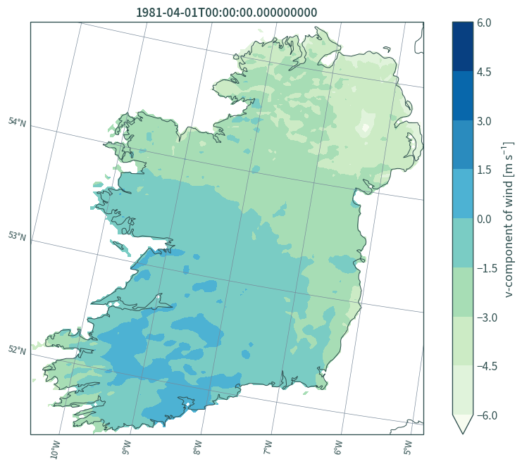
"34_105_10_0", # v-component of 10 m wind
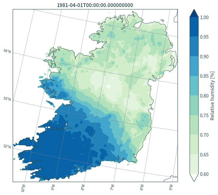
"52_105_2_0", # 2 m relative humidity
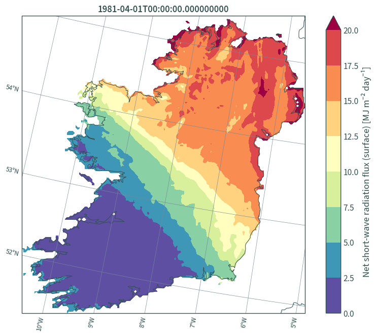
"111_105_0_4", # net shortwave irradiance
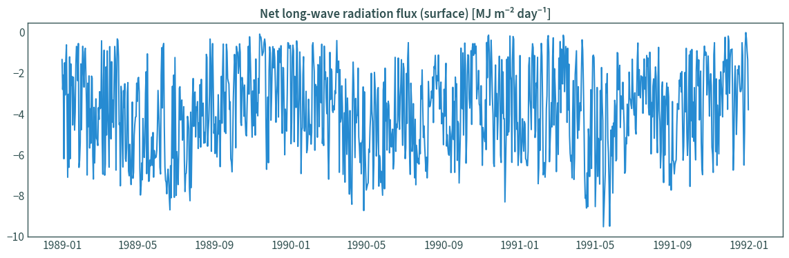
"112_105_0_4", # net longwave irradiance
]
# dictionary to store Xarray datasets
ds = {}
for var in var_dirs:
    ds[var] = xr.open_mfdataset(
        glob.glob(os.path.join(DATA_DIR, f"MERA_{var}_day.nc")),
        chunks="auto",
        decode_coords="all",
    )
# obtain CRS info
data_crs = ds["1_105_0_0"].rio.crs
# drop the height dimension from the datasets
for v in var_dirs:
    ds[v] = ds[v].isel(height=0)
Visualise the variables#
# Moorepark, Fermoy met station coords
LON, LAT = -8.26389, 52.16389
# transform coordinates from lon/lat to Lambert Conformal Conic
XLON, YLAT = cplt.projection_lambert_conformal.transform_point(
    x=LON, y=LAT, src_crs=ccrs.PlateCarree()
)
def plot_map(data, var, cmap="Spectral_r"):
    """
    Helper function for plotting maps
    """

    plt.figure(figsize=(9, 7))
    ax = plt.axes(projection=cplt.projection_lambert_conformal)
    data.isel(time=120)[var].plot.contourf(
        ax=ax,
        robust=True,
        x="x",
        y="y",
        levels=10,
        transform=cplt.projection_lambert_conformal,
        cmap=cmap,
        cbar_kwargs={
            "label": (
                data[var].attrs["long_name"]
                + " ["
                + data[var].attrs["units"]
                + "]"
            )
        },
    )
    ax.gridlines(
        draw_labels=dict(bottom="x", left="y"),
        color="lightslategrey",
        linewidth=0.5,
        x_inline=False,
        y_inline=False,
    )
    ax.coastlines(resolution="10m", color="darkslategrey", linewidth=0.75)
    ax.set_title(str(data.isel(time=90)["time"].values))
    plt.tight_layout()
    plt.show()
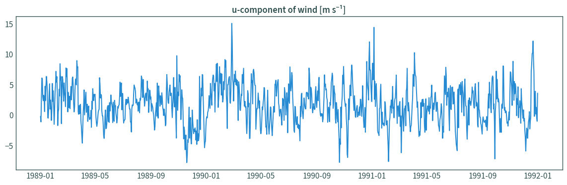
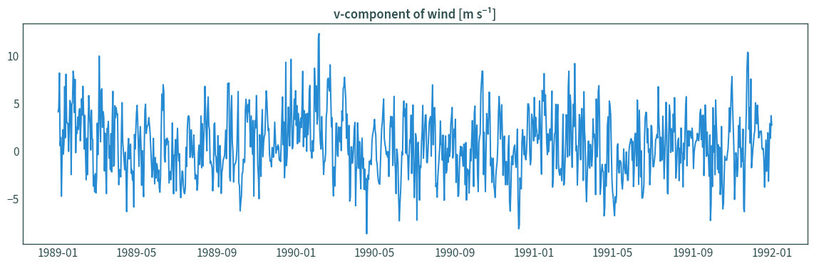
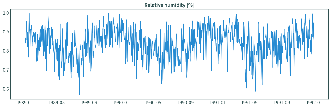
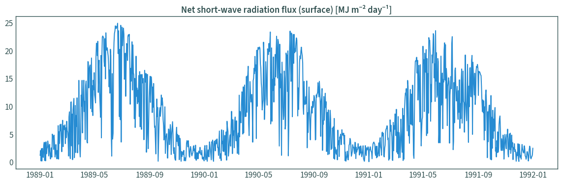
def plot_ts(data, var):
    """
    Helper function for plotting time series
    """

    plt.figure(figsize=(12, 4))
    data_ts = data.sel({"x": XLON, "y": YLAT}, method="nearest")
    data_ts = data_ts.sel(time=slice("1989", "1991"))
    plt.plot(data_ts["time"], data_ts[var])
    plt.title(
        data[var].attrs["long_name"] + " [" + data[var].attrs["units"] + "]"
    )
    plt.tight_layout()
    plt.show()
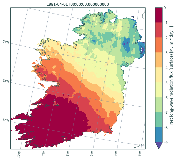
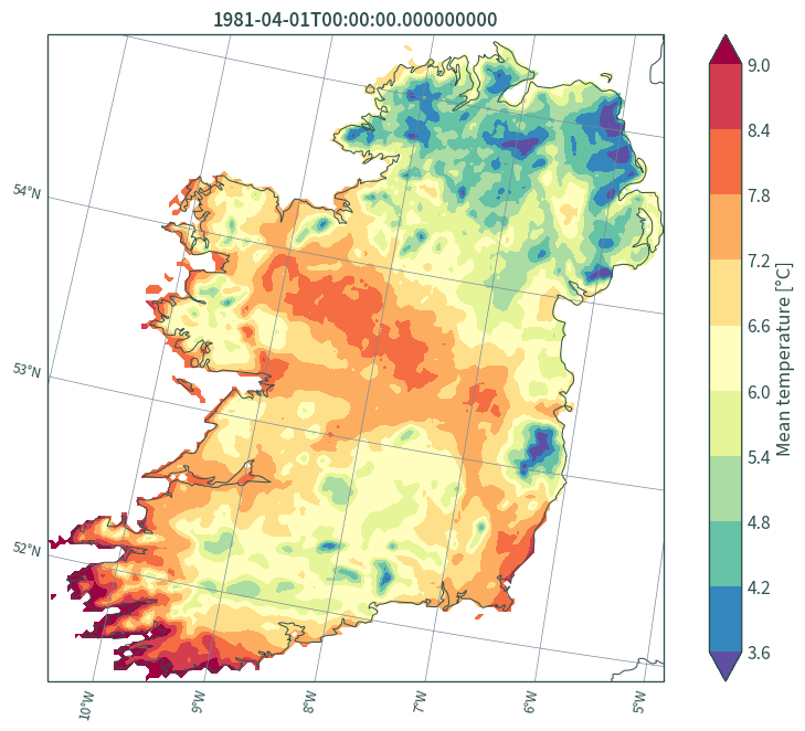
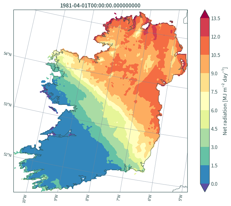
for v in var_dirs:
    var = list(ds[v].data_vars)[0]
    plot_map(ds[v], var, climag_plot.colormap_configs(var))
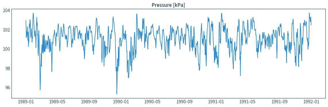
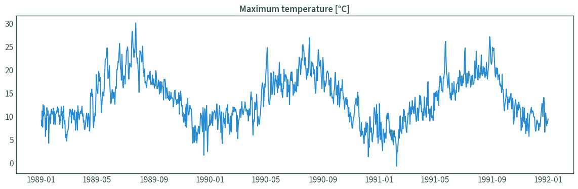
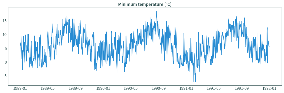
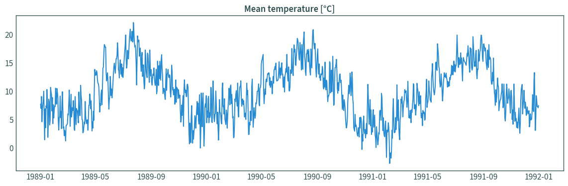
for v in var_dirs:
    var = list(ds[v].data_vars)[0]
    plot_ts(ds[v], var)
Prepare variables to calculate ET#
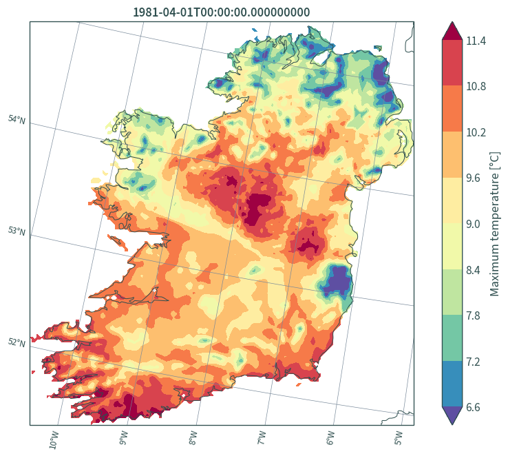
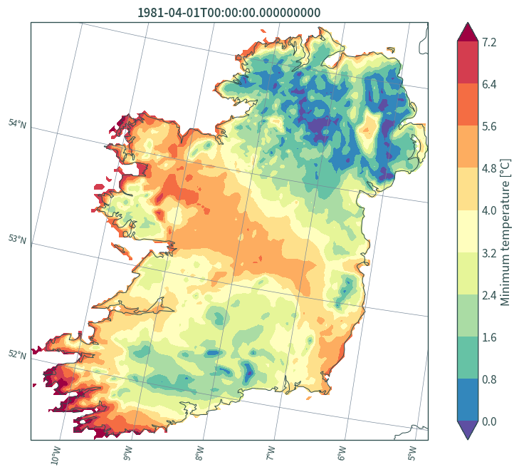
Mean air temperature#
Due to the non-linearity of humidity data required in the FAO Penman-Monteith equation, the vapour pressure for a certain period should be computed as the mean between the vapour pressure at the daily maximum and minimum air temperatures of that period.
The daily maximum air temperature and daily minimum air temperature are, respectively, the maximum and minimum air temperature observed during the 24-hour period, beginning at midnight.
The mean daily air temperature is only employed in the FAO Penman-Monteith equation to calculate the slope of the saturation vapour pressure curves and the impact of mean air density as the effect of temperature variations on the value of the climatic parameter is small in these cases.
For standardisation, the mean temperature for 24-hour periods is defined as the mean of the daily maximum and minimum temperatures rather than as the average of hourly temperature measurements.
Equation (9) in Allen et al. (1998), p.33
\(T_{mean}\): mean air temperature at 2 m height [°C]
\(T_{max}\): maximum air temperature at 2 m height [°C]
\(T_{min}\): minimum air temperature at 2 m height [°C]
t_mean = xr.combine_by_coords(
    [ds["15_105_2_2"], ds["16_105_2_2"]], combine_attrs="drop_conflicts"
)
t_mean = t_mean.assign(t_mean=(t_mean["tmax"] + t_mean["tmin"]) / 2)
t_mean["t_mean"].attrs["units"] = "°C"
t_mean["t_mean"].attrs["long_name"] = "Mean temperature"
t_mean = t_mean.drop_vars(["tmax", "tmin"])
t_mean.rio.write_crs(data_crs, inplace=True)
<xarray.Dataset>
Dimensions:            (x: 158, y: 166, time: 9131)
Coordinates:
  * x                  (x) float64 4.15e+05 4.175e+05 ... 8.05e+05 8.075e+05
  * y                  (y) float64 4.075e+05 4.1e+05 ... 8.175e+05 8.2e+05
    height             float64 2.0
    Lambert_Conformal  int64 0
  * time               (time) datetime64[ns] 1981-01-01 ... 2005-12-31
    spatial_ref        int64 0
Data variables:
    t_mean             (time, y, x) float32 dask.array<chunksize=(4871, 85, 81), meta=np.ndarray>
Attributes:
    CDI:          Climate Data Interface version 2.0.5 (https://mpimet.mpg.de...
    Conventions:  CF-1.6
CDO: Climate Data Operators version 2.0.5 (https://mpimet.mpg.de...plot_map(t_mean, "t_mean")
plot_ts(t_mean, "t_mean")
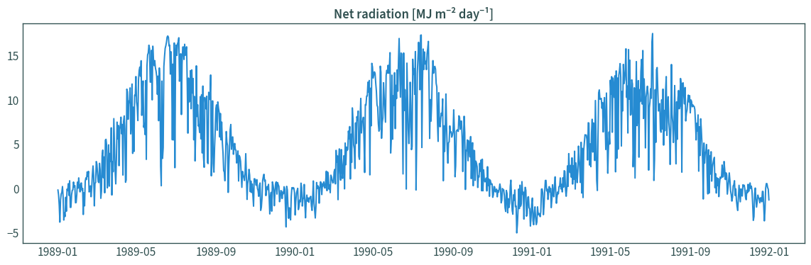
Net radiation#
The net radiation is the difference between the incoming net shortwave radiation and the outgoing net longwave radiation.
Equation (40) in Allen et al. (1998), p. 53
\(R_n\): net radiation at the crop surface [MJ m⁻² day⁻¹]
\(R_{ns}\): incoming net shortwave radiation [MJ m⁻² day⁻¹]
\(R_{nl}\): outgoing net longwave radiation [MJ m⁻² day⁻¹]
r_n = xr.combine_by_coords(
    [ds["111_105_0_4"], ds["112_105_0_4"]], combine_attrs="drop_conflicts"
)
# since both are incoming, they must be added, not subtracted
r_n = r_n.assign(r_n=r_n["nswrs"] + r_n["nlwrs"])
r_n["r_n"].attrs["units"] = "MJ m⁻² day⁻¹"
r_n["r_n"].attrs["long_name"] = "Net radiation"
r_n = r_n.drop_vars(["nswrs", "nlwrs"])
r_n.rio.write_crs(data_crs, inplace=True)
<xarray.Dataset>
Dimensions:            (x: 158, y: 166, time: 9131)
Coordinates:
  * x                  (x) float64 4.15e+05 4.175e+05 ... 8.05e+05 8.075e+05
  * y                  (y) float64 4.075e+05 4.1e+05 ... 8.175e+05 8.2e+05
    height             float64 0.0
    Lambert_Conformal  int64 0
  * time               (time) datetime64[ns] 1981-01-01 ... 2005-12-31
    spatial_ref        int64 0
Data variables:
    r_n                (time, y, x) float32 dask.array<chunksize=(4871, 85, 81), meta=np.ndarray>
Attributes:
    CDI:          Climate Data Interface version 2.0.5 (https://mpimet.mpg.de...
    Conventions:  CF-1.6
CDO: Climate Data Operators version 2.0.5 (https://mpimet.mpg.de...plot_map(r_n, "r_n")
plot_ts(r_n, "r_n")
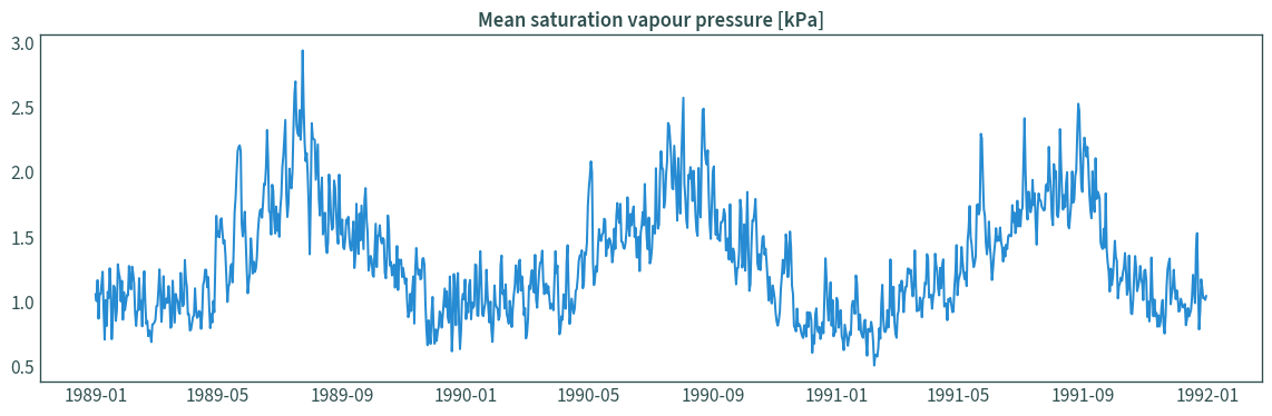
Saturation vapour pressure#
Equation (11) in Allen et al. (1998), p. 36
\(e^o(T)\): saturation vapour pressure at the air temperature T [kPa]
\(T\): air temperature [°C]
Equation (12) in Allen et al. (1998), p. 36
\(e_s\): mean saturation vapour pressure [kPa]
\(e^o(T_{max})\): saturation vapour pressure at the maximum air temperature [kPa]
\(e^o(T_{min})\): saturation vapour pressure at the minimum air temperature [kPa]
e_s = xr.combine_by_coords(
    [ds["15_105_2_2"], ds["16_105_2_2"]], combine_attrs="drop_conflicts"
)
e_s = e_s.assign(
    e_s_tmax=0.6108 * np.exp((17.27 * e_s["tmax"]) / (e_s["tmax"] + 237.3))
)
e_s = e_s.assign(
    e_s_tmin=0.6108 * np.exp((17.27 * e_s["tmin"]) / (e_s["tmin"] + 237.3))
)
e_s = e_s.assign(e_s=(e_s["e_s_tmax"] + e_s["e_s_tmin"]) / 2)
e_s["e_s"].attrs["units"] = "kPa"
e_s["e_s"].attrs["long_name"] = "Mean saturation vapour pressure"
e_s = e_s.drop_vars(["tmax", "tmin", "e_s_tmax", "e_s_tmin"])
e_s.rio.write_crs(data_crs, inplace=True)
<xarray.Dataset>
Dimensions:            (x: 158, y: 166, time: 9131)
Coordinates:
  * x                  (x) float64 4.15e+05 4.175e+05 ... 8.05e+05 8.075e+05
  * y                  (y) float64 4.075e+05 4.1e+05 ... 8.175e+05 8.2e+05
    height             float64 2.0
    Lambert_Conformal  int64 0
  * time               (time) datetime64[ns] 1981-01-01 ... 2005-12-31
    spatial_ref        int64 0
Data variables:
    e_s                (time, y, x) float32 dask.array<chunksize=(4871, 85, 81), meta=np.ndarray>
Attributes:
    CDI:          Climate Data Interface version 2.0.5 (https://mpimet.mpg.de...
    Conventions:  CF-1.6
CDO: Climate Data Operators version 2.0.5 (https://mpimet.mpg.de...plot_map(e_s, "e_s", "flare")
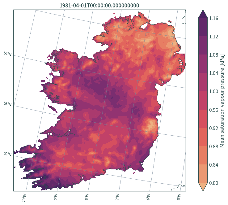
plot_ts(e_s, "e_s")
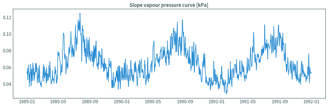
Slope vapour pressure curve#
The slope of the relationship between saturation vapour pressure and temperature.
Equation (13) in Allen et al. (1998), p. 37
\(Δ\): slope vapour pressure curve [kPa °C⁻¹]
\(T\): mean air temperature at 2 m height [°C]
In the FAO Penman-Monteith equation, where \(∆\) occurs in the numerator and denominator, the slope of the vapour pressure curve is calculated using mean air temperature.
delta = t_mean.copy()
delta = delta.assign(
    delta=(
        4098
        * (
            0.6108
            * np.exp((17.27 * delta["t_mean"]) / (delta["t_mean"] + 237.3))
        )
        / np.power((delta["t_mean"] + 273.3), 2)
    )
)
delta["delta"].attrs["units"] = "kPa"
delta["delta"].attrs["long_name"] = "Slope vapour pressure curve"
delta = delta.drop_vars(["t_mean"])
delta.rio.write_crs(data_crs, inplace=True)
<xarray.Dataset>
Dimensions:            (x: 158, y: 166, time: 9131)
Coordinates:
  * x                  (x) float64 4.15e+05 4.175e+05 ... 8.05e+05 8.075e+05
  * y                  (y) float64 4.075e+05 4.1e+05 ... 8.175e+05 8.2e+05
    height             float64 2.0
    Lambert_Conformal  int64 0
  * time               (time) datetime64[ns] 1981-01-01 ... 2005-12-31
    spatial_ref        int64 0
Data variables:
    delta              (time, y, x) float32 dask.array<chunksize=(4871, 85, 81), meta=np.ndarray>
Attributes:
    CDI:          Climate Data Interface version 2.0.5 (https://mpimet.mpg.de...
    Conventions:  CF-1.6
CDO: Climate Data Operators version 2.0.5 (https://mpimet.mpg.de...plot_map(delta, "delta", "flare")
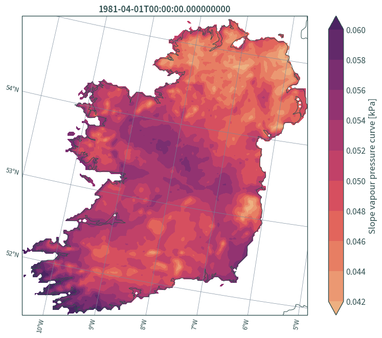
plot_ts(delta, "delta")
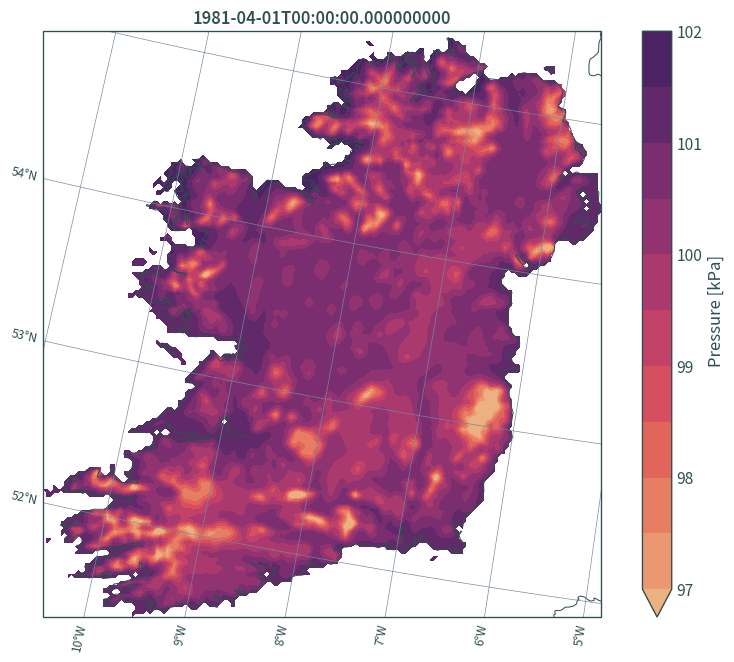
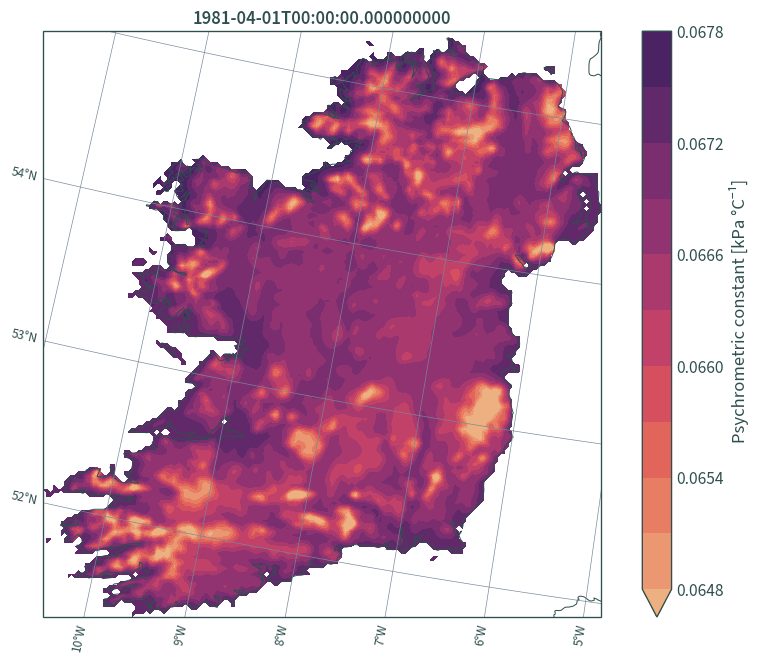
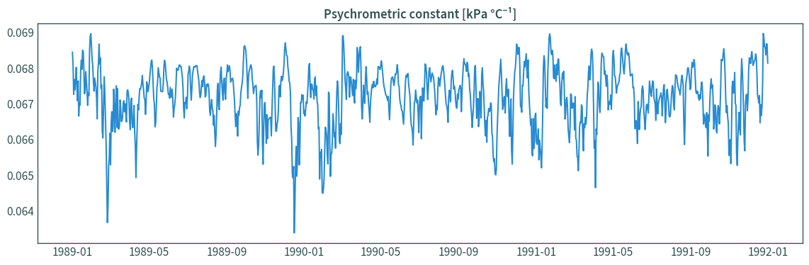
Psychrometric constant#
The psychrometric constant is the ratio of specific heat of moist air at constant pressure to latent heat of vaporisation of water. It can be estimated from atmospheric pressure.
This method assumes that the air is saturated with water vapour at the minimum daily temperature.
Equation (8) in Allen et al (1998), p. 32
\(γ = 0.665 \times 10^{-3} \times P\)
\(γ\): psychrometric constant [kPa °C⁻¹]
\(P\): atmospheric pressure [kPa]
gamma = ds["1_105_0_0"].copy()
gamma = gamma.assign(gamma=0.665 / 1000 * gamma["pres"])
gamma["gamma"].attrs["units"] = "kPa °C⁻¹"
gamma["gamma"].attrs["long_name"] = "Psychrometric constant"
gamma = gamma.drop_vars(["pres"])
gamma.rio.write_crs(data_crs, inplace=True)
<xarray.Dataset>
Dimensions:            (x: 158, y: 166, time: 9131)
Coordinates:
  * x                  (x) float64 4.15e+05 4.175e+05 ... 8.05e+05 8.075e+05
  * y                  (y) float64 4.075e+05 4.1e+05 ... 8.175e+05 8.2e+05
    height             float64 0.0
    Lambert_Conformal  int64 ...
  * time               (time) datetime64[ns] 1981-01-01 ... 2005-12-31
    spatial_ref        int64 0
Data variables:
    gamma              (time, y, x) float32 dask.array<chunksize=(4871, 85, 81), meta=np.ndarray>
Attributes:
    CDI:          Climate Data Interface version 2.0.5 (https://mpimet.mpg.de...
    Conventions:  CF-1.6
    history:      Wed Mar 22 15:36:57 2023: cdo -s -f nc4c -shifttime,-3hour ...
CDO: Climate Data Operators version 2.0.5 (https://mpimet.mpg.de...plot_map(gamma, "gamma", "flare")
plot_ts(gamma, "gamma")
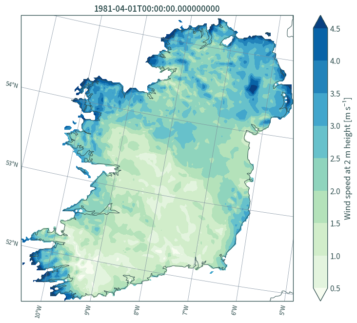
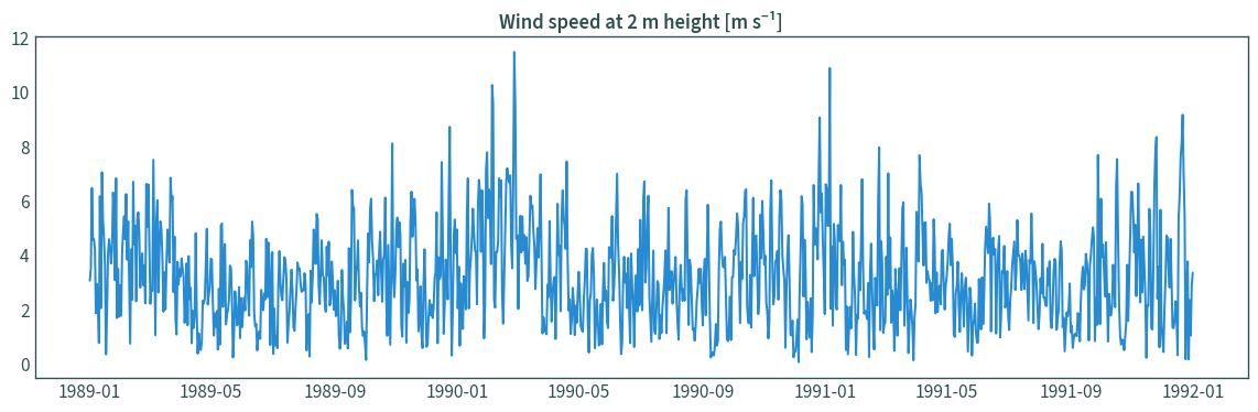
Wind speed#
Calculate the wind speed using u- and v-components.
http://colaweb.gmu.edu/dev/clim301/lectures/wind/wind-uv
\(w\): wind speed [m s⁻¹]
\(u\): u-component of wind speed [m s⁻¹]
\(v\): v-component of wind speed [m s⁻¹]
If not measured at 2 m height, convert wind speed measured at different heights above the soil surface to wind speed at 2 m above the surface, assuming a short grass surface.
Equation (47) in Allen et al (1998), p. 56
\(w_2\): wind speed at 2 m height [m s⁻¹]
\(w_z\): measured wind speed at z m above ground surface [m s⁻¹]
\(z\): height of measurement above ground surface [m]
w_2 = xr.combine_by_coords(
    [ds["33_105_10_0"], ds["34_105_10_0"]], combine_attrs="drop_conflicts"
)
w_2 = w_2.assign(w=np.hypot(w_2["u"], w_2["v"]))
w_2 = w_2.assign(w_2=w_2["w"] * (4.87 / np.log((67.8 * 10.0) - 5.42)))
w_2["w_2"].attrs["units"] = "m s⁻¹"
w_2["w_2"].attrs["long_name"] = "Wind speed at 2 m height"
w_2 = w_2.drop_vars(["u", "v", "w"])
w_2.rio.write_crs(data_crs, inplace=True)
<xarray.Dataset>
Dimensions:            (x: 158, y: 166, time: 9131)
Coordinates:
  * x                  (x) float64 4.15e+05 4.175e+05 ... 8.05e+05 8.075e+05
  * y                  (y) float64 4.075e+05 4.1e+05 ... 8.175e+05 8.2e+05
    height             float64 10.0
    Lambert_Conformal  int64 0
  * time               (time) datetime64[ns] 1981-01-01 ... 2005-12-31
    spatial_ref        int64 0
Data variables:
    w_2                (time, y, x) float32 dask.array<chunksize=(4871, 85, 81), meta=np.ndarray>
Attributes:
    CDI:          Climate Data Interface version 2.0.5 (https://mpimet.mpg.de...
    Conventions:  CF-1.6
CDO: Climate Data Operators version 2.0.5 (https://mpimet.mpg.de...plot_map(w_2, "w_2", "GnBu")
plot_ts(w_2, "w_2")
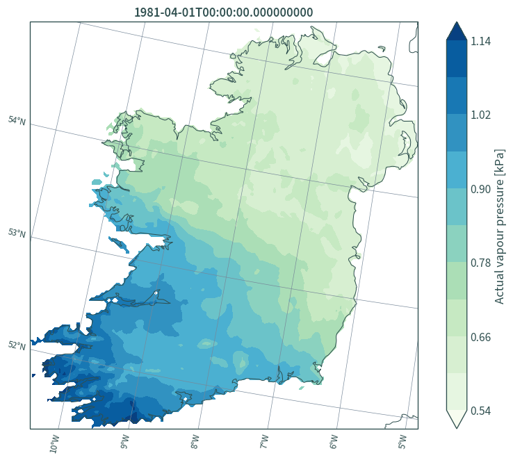
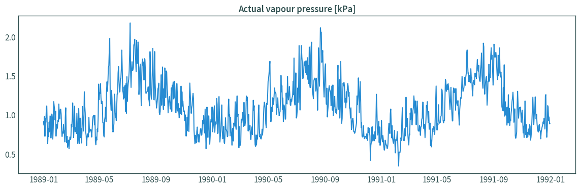
Actual vapour pressure#
In the absence of dewpoint temperature, or psychrometric data (i.e. wet and dry bulb temperatures), or maximum (and minimum) relative humidity, the mean relative humidity is used to calculate the actual vapour pressure.
Equation (19) in Allen et al. (1998), p. 39
\(e_a\): actual vapour pressure [kPa]
\(RH_{mean}\): mean relative humidity [%]
\(e_s\): saturation vapour pressure [kPa]
e_a = xr.combine_by_coords(
    [ds["52_105_2_0"], e_s], combine_attrs="drop_conflicts"
)
e_a = e_a.assign(e_a=e_a["r"] * e_a["e_s"])  # "r" ranges from 0.0 - 1.0
e_a["e_a"].attrs["units"] = "kPa"
e_a["e_a"].attrs["long_name"] = "Actual vapour pressure"
e_a = e_a.drop_vars(["r", "e_s"])
e_a.rio.write_crs(data_crs, inplace=True)
<xarray.Dataset>
Dimensions:            (x: 158, y: 166, time: 9131)
Coordinates:
  * x                  (x) float64 4.15e+05 4.175e+05 ... 8.05e+05 8.075e+05
  * y                  (y) float64 4.075e+05 4.1e+05 ... 8.175e+05 8.2e+05
    height             float64 2.0
    Lambert_Conformal  int64 0
  * time               (time) datetime64[ns] 1981-01-01 ... 2005-12-31
    spatial_ref        int64 0
Data variables:
    e_a                (time, y, x) float32 dask.array<chunksize=(4871, 85, 81), meta=np.ndarray>
Attributes:
    CDI:          Climate Data Interface version 2.0.5 (https://mpimet.mpg.de...
    Conventions:  CF-1.6
    CDO:          Climate Data Operators version 2.0.5 (https://mpimet.mpg.de...
history: Wed Mar 22 15:37:24 2023: cdo -s -f nc4c -shifttime,-3hour ...plot_map(e_a, "e_a", "GnBu")
plot_ts(e_a, "e_a")
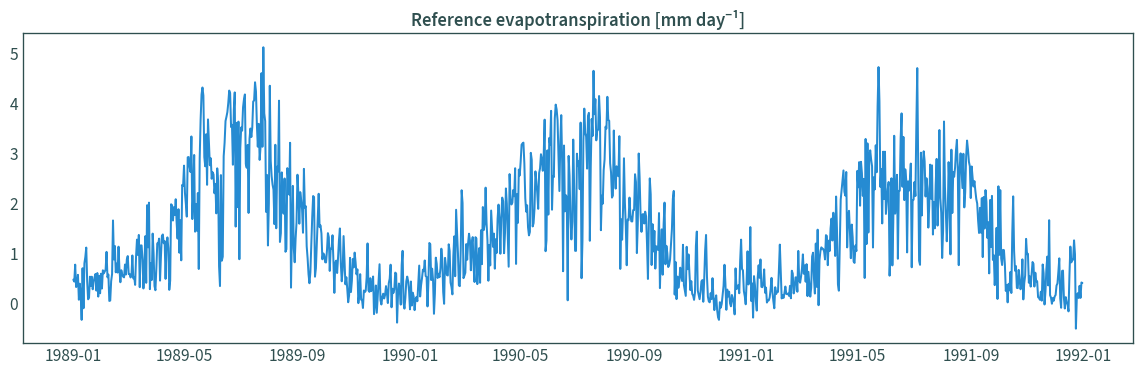
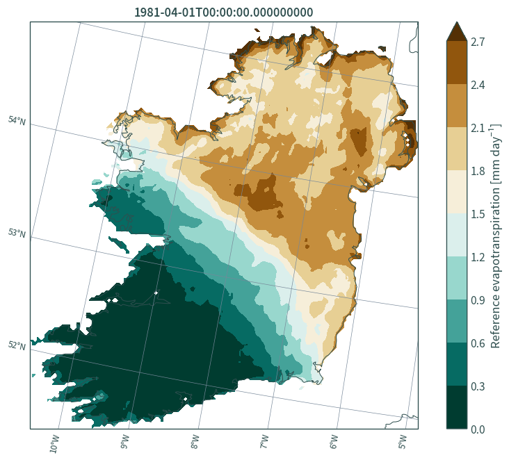
Calculate evapotranspiration#
The FAO Penman-Monteith equation.
Equation (6) in Allen et al. (1998), p. 24
\(ET_o\): reference evapotranspiration [mm day⁻¹]
\(Δ\): slope vapour pressure curve [kPa °C⁻¹]
\(R_n\): net radiation at the crop surface [MJ m⁻² day⁻¹]
\(G\): soil heat flux density [MJ m⁻² day⁻¹]
\(γ\): psychrometric constant [kPa °C⁻¹]
\(T\): mean daily air temperature at 2 m height [°C]
\(w_2\): wind speed at 2 m height [m s⁻¹]
\(e_s\): saturation vapour pressure [kPa]
\(e_a\): actual vapour pressure [kPa]
The soil heat flux is small compared to net radiation, particularly when the surface is covered by vegetation. As the magnitude of the day heat flux beneath the grass reference surface is relatively small, it may be ignored.
Equation (42) in Allen et al. (1998), p. 54
eto = xr.combine_by_coords(
    [delta, gamma, r_n, t_mean, w_2, e_s, e_a],
    combine_attrs="drop_conflicts",
    compat="override",
)
eto = eto.assign(
    PET=(
        (
            (0.408 * eto["delta"] * eto["r_n"])
            + eto["gamma"]
            * (900 / (eto["t_mean"] + 273))
            * eto["w_2"]
            * (eto["e_s"] - eto["e_a"])
        )
        / (eto["delta"] + eto["gamma"] * (1 + 0.34 * eto["w_2"]))
    )
)
eto["PET"].attrs["units"] = "mm day⁻¹"
eto["PET"].attrs["long_name"] = "Reference evapotranspiration"
eto = eto.drop_vars(["delta", "gamma", "e_a", "e_s", "r_n", "t_mean", "w_2"])
eto.rio.write_crs(data_crs, inplace=True)
<xarray.Dataset>
Dimensions:            (x: 158, y: 166, time: 9131)
Coordinates:
  * x                  (x) float64 4.15e+05 4.175e+05 ... 8.05e+05 8.075e+05
  * y                  (y) float64 4.075e+05 4.1e+05 ... 8.175e+05 8.2e+05
    height             float64 2.0
    Lambert_Conformal  int64 0
  * time               (time) datetime64[ns] 1981-01-01 ... 2005-12-31
    spatial_ref        int64 0
Data variables:
    PET                (time, y, x) float32 dask.array<chunksize=(4871, 85, 81), meta=np.ndarray>
Attributes:
    CDI:          Climate Data Interface version 2.0.5 (https://mpimet.mpg.de...
    Conventions:  CF-1.6
CDO: Climate Data Operators version 2.0.5 (https://mpimet.mpg.de...plot_map(eto, "PET", "BrBG_r")
plot_ts(eto, "PET")