Compare grass growth time series using MERA for each county at a weekly frequency

import os
import matplotlib.pyplot as plt
import pandas as pd
import seaborn as sns
import statsmodels.api as sm
from sklearn.metrics import mean_squared_error
import geopandas as gpd

df1 = pd.read_csv(
    os.path.join(
        "data", "grass_growth", "PastureBaseIreland", "pasturebase_cleaned.csv"
    )
)
df2 = pd.read_csv(
    os.path.join(
        "data", "grass_growth", "GrassCheckNI", "grasscheck_cleaned.csv"
    )
)
df = pd.concat([df1, df2])
df_p = pd.pivot_table(
    df[["time", "county", "value"]],
    values="value",
    index=["time"],
    columns=["county"],
)
df_p.index = pd.to_datetime(df_p.index)

mera = pd.read_csv(
    os.path.join("data", "ModVege", "growth", "MERA_growth_week_pasture.csv")
)
mera.rename(columns={"COUNTY": "county", "mean": "value"}, inplace=True)
mera["county"] = mera["county"].str.title()
mera_p = pd.pivot_table(
    mera, values="value", index=["time"], columns=["county"]
)
mera_p.index = pd.to_datetime(mera_p.index)

counties = list(df_p)

df["data"] = "Measured"
mera["data"] = "Simulated"
data_all = pd.concat([df, mera])
data_all.set_index("time", inplace=True)
data_all.index = pd.to_datetime(data_all.index)
# data_all_p = pd.pivot_table(
#     data_all[["county", "value", "data"]],
#     values="value", index=["time"], columns=["county", "data"]
# )
# data_all_p.resample("Y").mean()

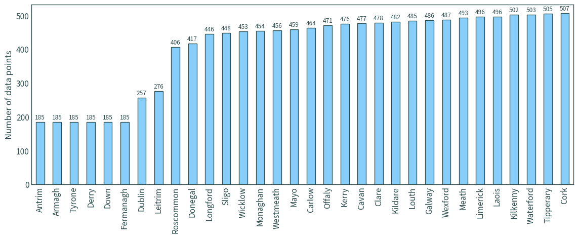
Number of data points

ax = (
    pd.DataFrame(df_p.count())
    .sort_values(by=0)
    .plot.bar(
        legend=False,
        figsize=(12, 5),
        color="lightskyblue",
        edgecolor="darkslategrey",
    )
)
ax.bar_label(ax.containers[0], padding=2)
plt.xlabel("")
plt.ylabel("Number of data points")
plt.tight_layout()
plt.show()

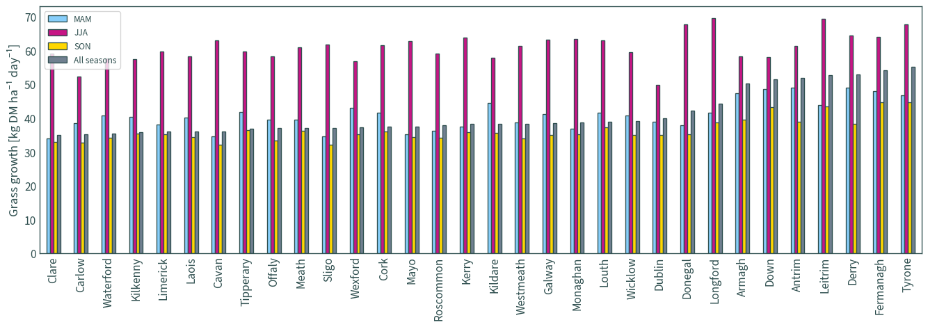
Measured averages

lta_all = pd.DataFrame(df_p.mean(), columns=["All seasons"]).sort_values(
    by="All seasons"
)

lta_mam = pd.DataFrame(
    df_p[
        (df_p.index.month == 3)
        | (df_p.index.month == 4)
        | (df_p.index.month == 5)
    ].mean(),
    columns=["MAM"],
).sort_values(by="MAM")

lta_jja = pd.DataFrame(
    df_p[
        (df_p.index.month == 6)
        | (df_p.index.month == 7)
        | (df_p.index.month == 8)
    ].mean(),
    columns=["JJA"],
).sort_values(by="JJA")

lta_son = pd.DataFrame(
    df_p[
        (df_p.index.month == 9)
        | (df_p.index.month == 10)
        | (df_p.index.month == 11)
    ].mean(),
    columns=["SON"],
).sort_values(by="SON")

pd.concat([lta_mam, lta_jja, lta_son, lta_all], axis=1).sort_values(
    by=["All seasons", "SON", "JJA", "MAM"]
).plot.bar(
    figsize=(14, 5),
    edgecolor="darkslategrey",
    color=["lightskyblue", "mediumvioletred", "gold", "slategrey"],
)
plt.xlabel("")
plt.ylabel("Grass growth [kg DM ha⁻¹ day⁻¹]")
plt.tight_layout()
plt.show()

pd.concat([lta_mam, lta_jja, lta_son, lta_all], axis=1).to_csv(
    os.path.join("data", "grass_growth", "average_growth.csv")
)

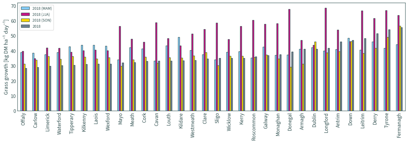
2018 averages

a2018_all = pd.DataFrame(
    df_p.loc["2018"].mean(), columns=["2018"]
).sort_values(by="2018")

a2018_mam = pd.DataFrame(
    df_p[
        (df_p.index.month == 3)
        | (df_p.index.month == 4)
        | (df_p.index.month == 5)
    ]
    .loc["2018"]
    .mean(),
    columns=["2018 (MAM)"],
).sort_values(by="2018 (MAM)")

a2018_jja = pd.DataFrame(
    df_p[
        (df_p.index.month == 6)
        | (df_p.index.month == 7)
        | (df_p.index.month == 8)
    ]
    .loc["2018"]
    .mean(),
    columns=["2018 (JJA)"],
).sort_values(by="2018 (JJA)")

a2018_son = pd.DataFrame(
    df_p[
        (df_p.index.month == 9)
        | (df_p.index.month == 10)
        | (df_p.index.month == 11)
    ]
    .loc["2018"]
    .mean(),
    columns=["2018 (SON)"],
).sort_values(by="2018 (SON)")

pd.concat([a2018_mam, a2018_jja, a2018_son, a2018_all], axis=1).sort_values(
    by=["2018", "2018 (SON)", "2018 (JJA)", "2018 (MAM)"]
).plot.bar(
    figsize=(14, 5),
    edgecolor="darkslategrey",
    color=["lightskyblue", "mediumvioletred", "gold", "slategrey"],
)
plt.xlabel("")
plt.ylabel("Grass growth [kg DM ha⁻¹ day⁻¹]")
plt.tight_layout()
plt.show()

pd.concat([a2018_mam, a2018_jja, a2018_son, a2018_all], axis=1).to_csv(
    os.path.join("data", "grass_growth", "average_growth_2018.csv")
)

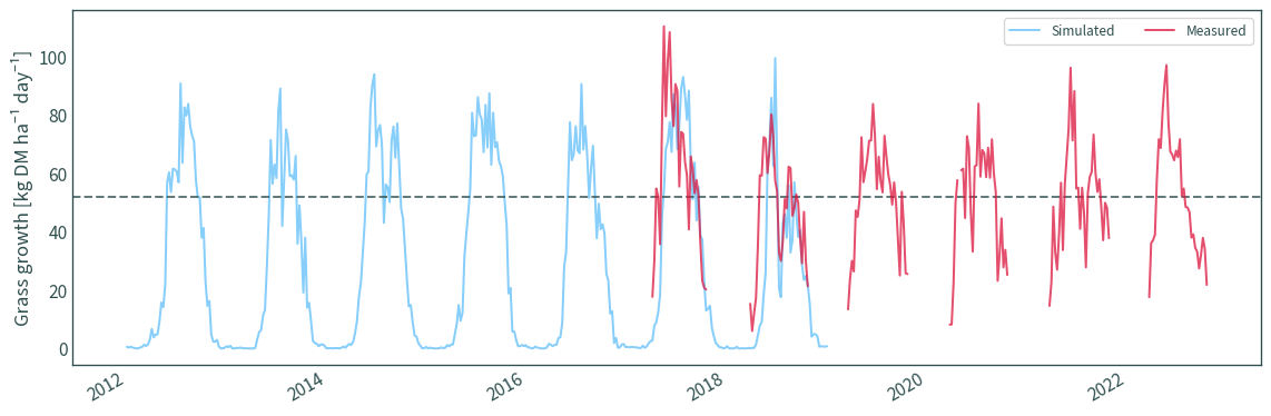
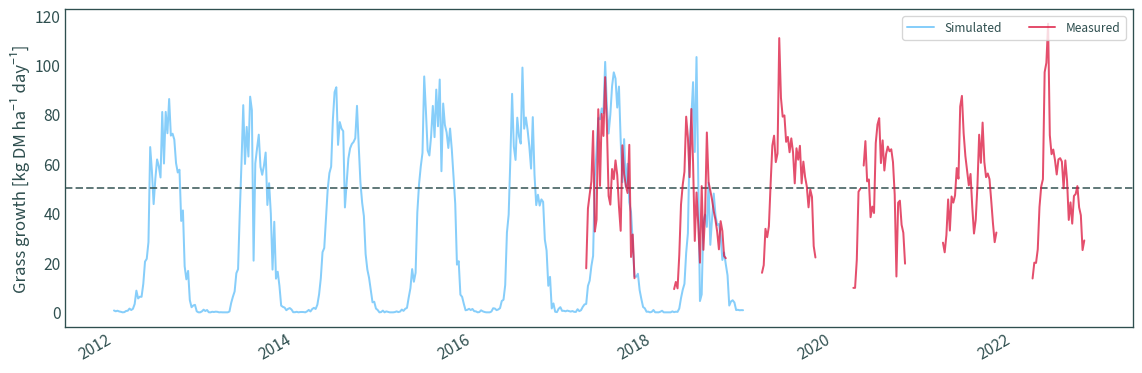
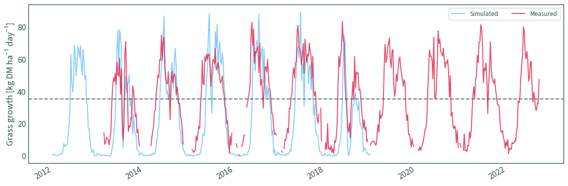
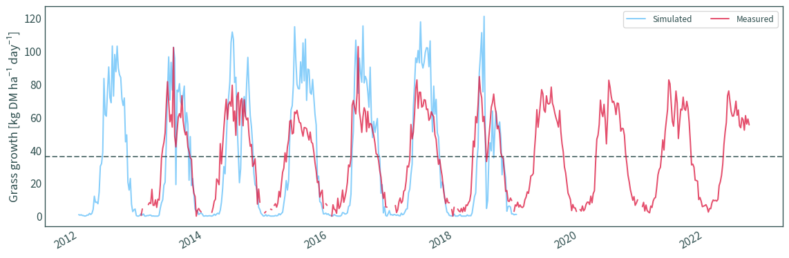
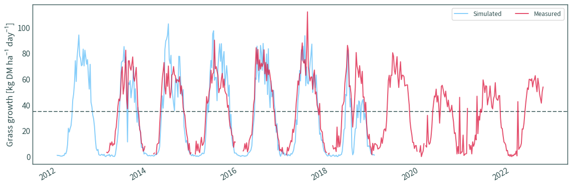
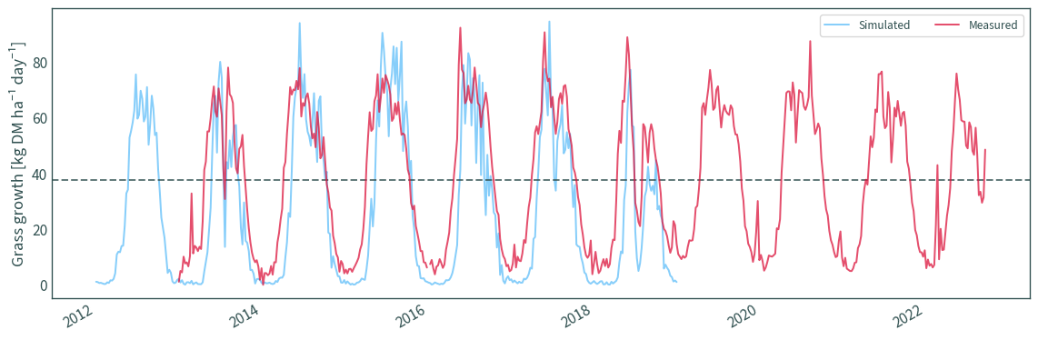
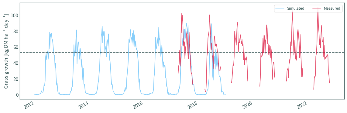
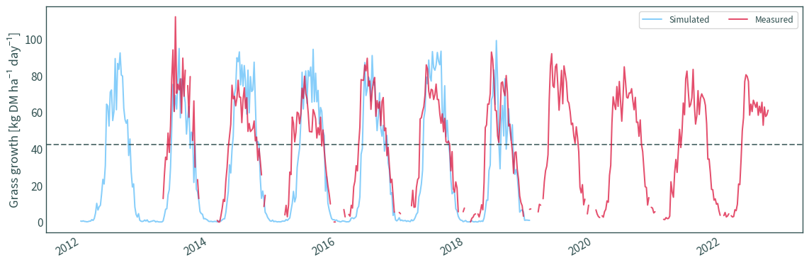
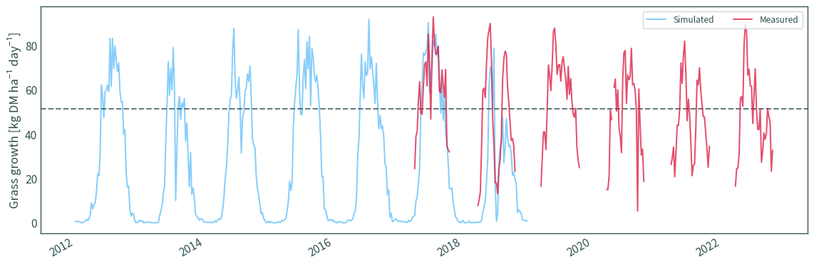
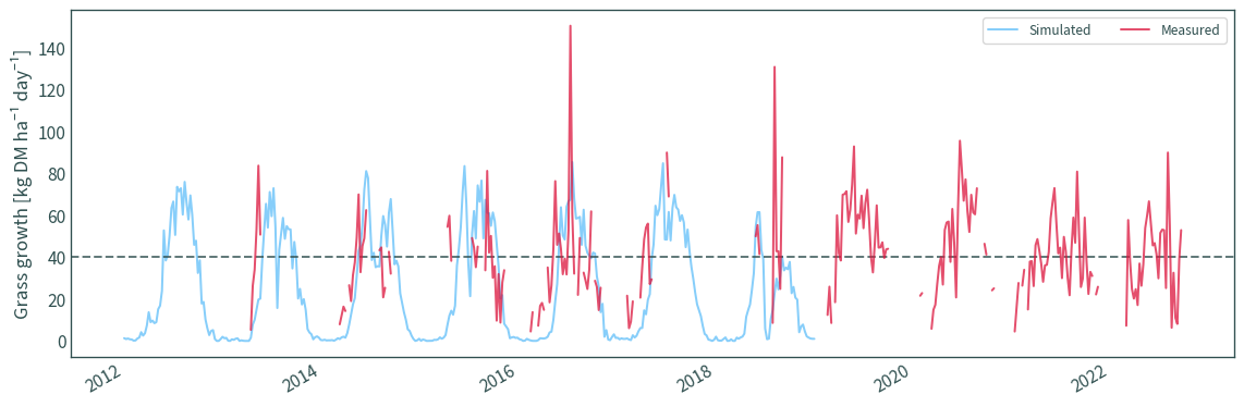
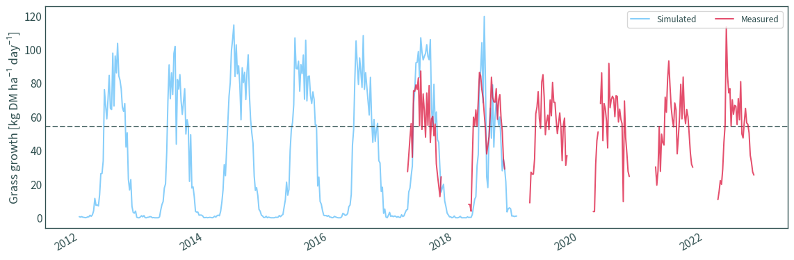
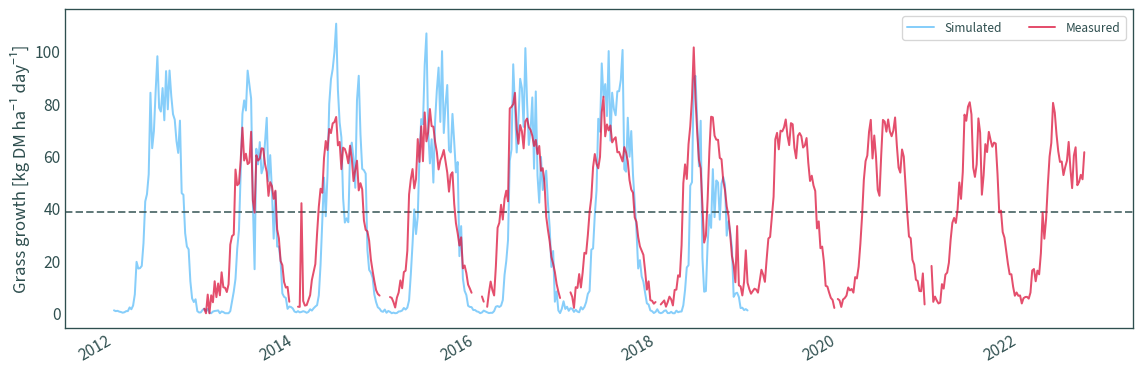
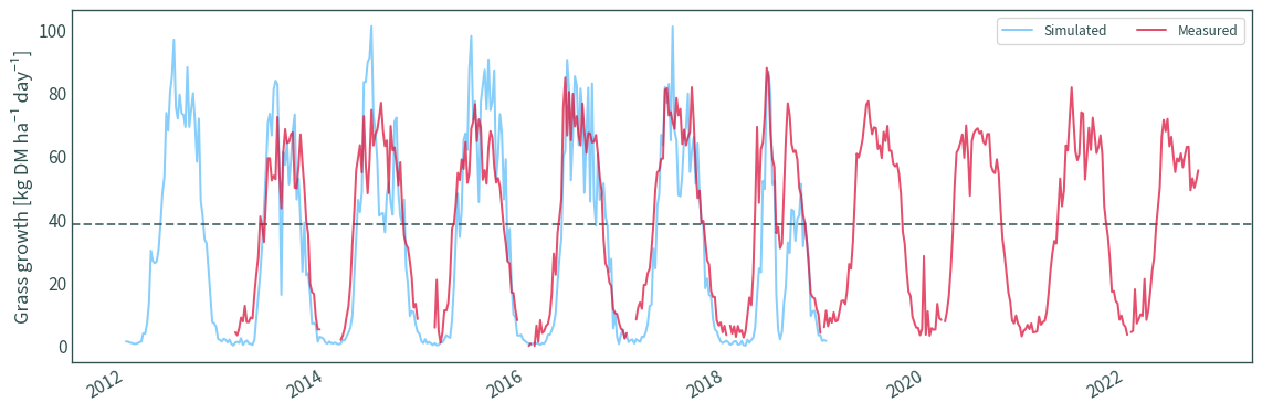
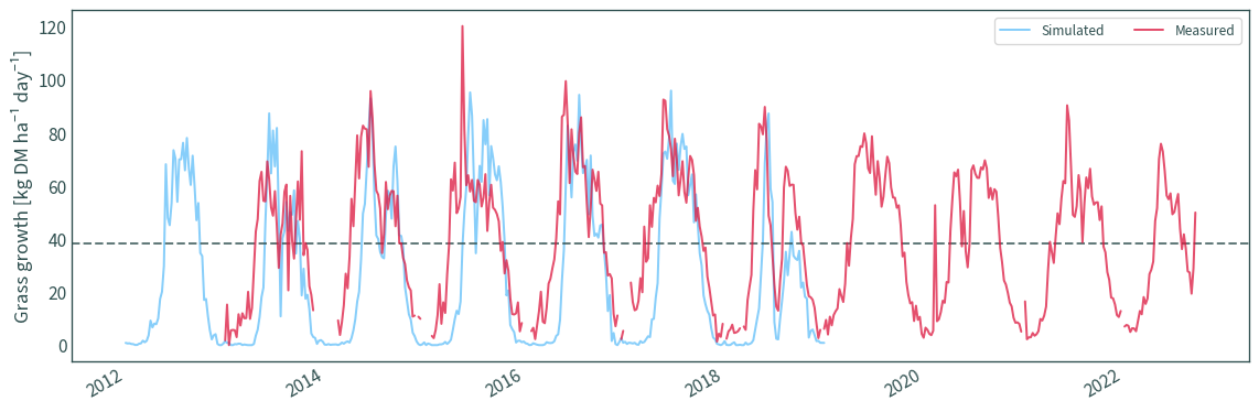
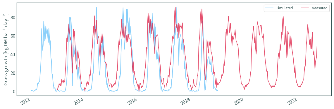
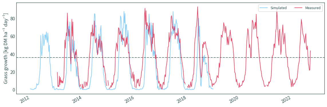
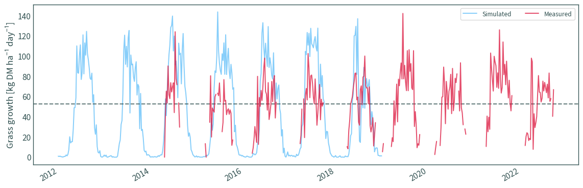
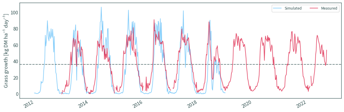
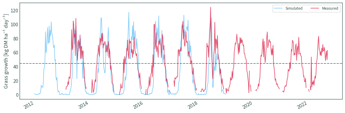
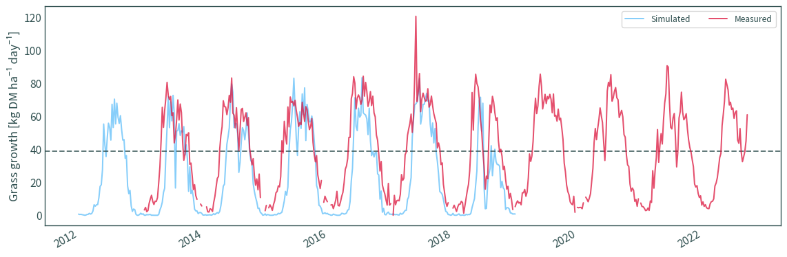
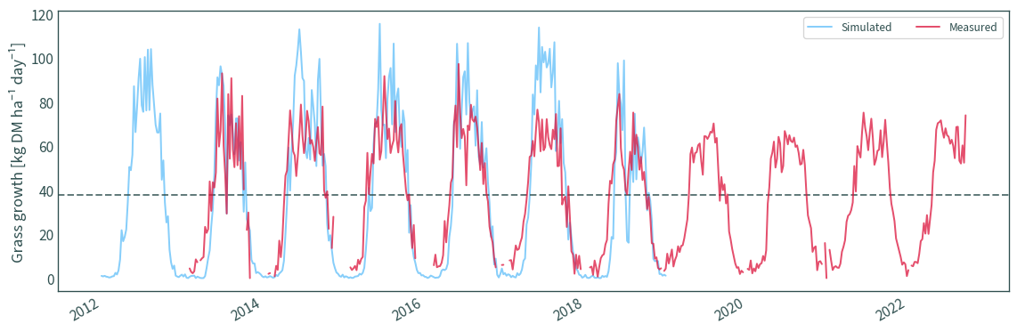
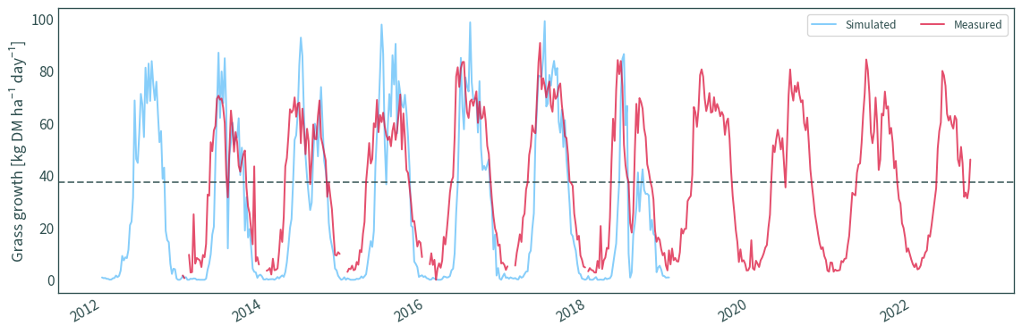
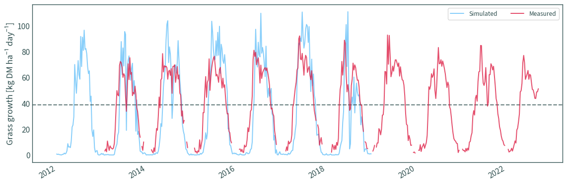
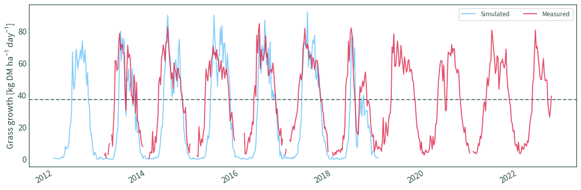
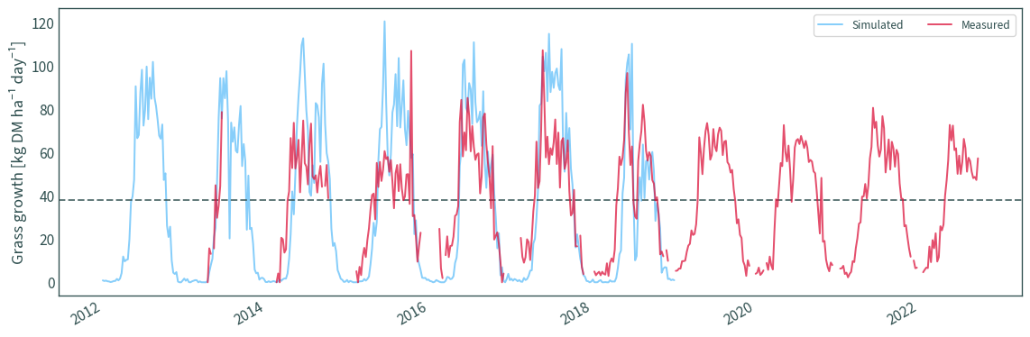
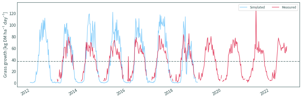
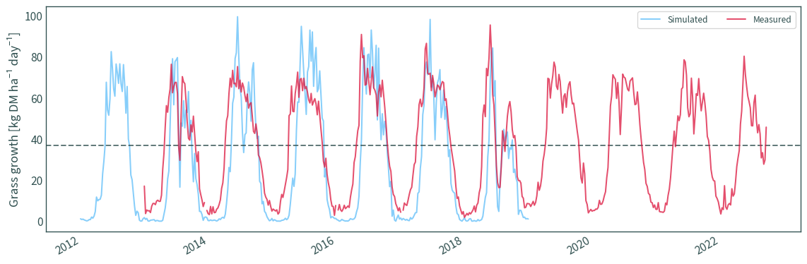
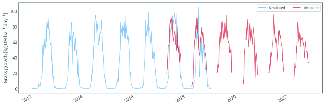
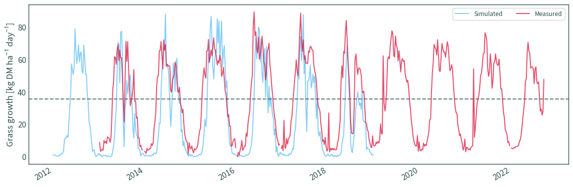
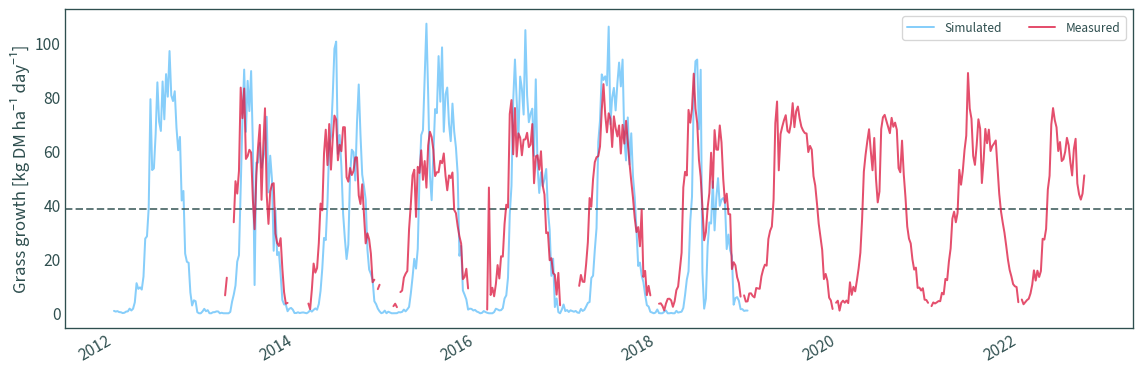
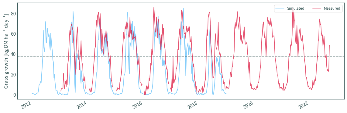
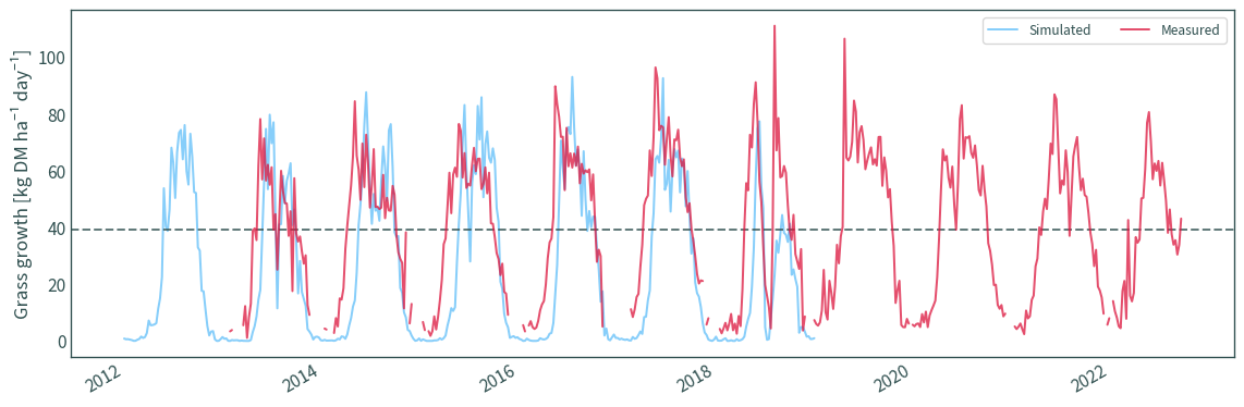
Weekly time series plots

for county in counties:
    plt.axhline(
        y=float(lta_all.loc[county]),
        linestyle="dashed",
        color="darkslategrey",
        alpha=0.75,  # label="Average (measured)"
    )
    # plt.axhline(
    #     y=float(lta_mam.loc[county]), linestyle="dotted",
    #     label="Average (MAM)", color="darkslategrey", alpha=.75
    # )
    # plt.axhline(
    #     y=float(lta_jja.loc[county]), linestyle="dashed",
    #     label="Average (JJA)", color="darkslategrey", alpha=.75
    # )
    # plt.axhline(
    #     y=float(lta_son.loc[county]), linestyle="dashdot",
    #     label="Average (SON)", color="darkslategrey", alpha=.75
    # )
    fig = mera_p["2012":"2019"][county].plot(
        figsize=(12, 4), label="Simulated", color="lightskyblue"
    )
    df_p[county].plot(
        ax=fig.axes, label="Measured", color="crimson", alpha=0.75
    )
    plt.legend(title=None, ncols=2, loc="upper right")
    plt.xlabel("")
    plt.ylabel("Grass growth [kg DM ha⁻¹ day⁻¹]")
    # plt.title(county)
    plt.tight_layout()
    print(county)
    plt.show()

Antrim

Armagh

Carlow

Cavan

Clare

Cork

Derry

Donegal

Down

Dublin

Fermanagh

Galway

Kerry

Kildare

Kilkenny

Laois

Leitrim

Limerick

Longford

Louth

Mayo

Meath

Monaghan

Offaly

Roscommon

Sligo

Tipperary

Tyrone

Waterford

Westmeath

Wexford

Wicklow

Stats

def get_plot_data(data_m, data_s, county, season=None):
    if county is None:
        plot_data = (
            pd.merge(
                data_m.melt(ignore_index=False)
                .reset_index()
                .set_index(["time", "county"])
                .rename(columns={"value": "Measured"}),
                data_s.melt(ignore_index=False)
                .reset_index()
                .set_index(["time", "county"])
                .rename(columns={"value": "Simulated"}),
                left_index=True,
                right_index=True,
            )
            .dropna()
            .reset_index()
            .set_index("time")
        )
    else:
        plot_data = pd.merge(
            data_m[[county]].rename(columns={county: "Measured"}),
            data_s[[county]].rename(columns={county: "Simulated"}),
            left_index=True,
            right_index=True,
        ).dropna()
    if season == "MAM":
        plot_data = plot_data[
            (plot_data.index.month == 3)
            | (plot_data.index.month == 4)
            | (plot_data.index.month == 5)
        ]
    elif season == "JJA":
        plot_data = plot_data[
            (plot_data.index.month == 6)
            | (plot_data.index.month == 7)
            | (plot_data.index.month == 8)
        ]
    elif season == "SON":
        plot_data = plot_data[
            (plot_data.index.month == 9)
            | (plot_data.index.month == 10)
            | (plot_data.index.month == 11)
        ]

    return plot_data

def rmse_by_county(data_m, data_s, counties=counties, season=None):
    if season:
        col_name = season
    else:
        col_name = "All seasons"
    rmse = pd.DataFrame(columns=["County", col_name])
    for i, county in enumerate(counties):
        plot_data = get_plot_data(data_m, data_s, county, season)
        rmse.loc[i] = [
            county,
            mean_squared_error(
                plot_data["Measured"], plot_data["Simulated"], squared=False
            ),
        ]
    plot_data = get_plot_data(data_m, data_s, county=None, season=season)
    rmse.loc[i + 1] = [
        "All counties",
        mean_squared_error(
            plot_data["Measured"], plot_data["Simulated"], squared=False
        ),
    ]
    # rmse.sort_values(by=[col_name], inplace=True)
    return rmse

def rmse_all(data_m, data_s):
    plot_data = pd.merge(
        pd.merge(
            pd.merge(
                rmse_by_county(df_p, mera_p, season="MAM"),
                rmse_by_county(df_p, mera_p, season="JJA"),
                on="County",
            ),
            rmse_by_county(df_p, mera_p, season="SON"),
            on="County",
        ),
        rmse_by_county(df_p, mera_p, season=None),
        on="County",
    )
    plot_data.sort_values(by="All seasons", inplace=True)
    return plot_data

def get_linear_regression(data_m, data_s, county, season=None):
    plot_data = get_plot_data(data_m, data_s, county, season)
    if county:
        print(county)

    x = plot_data["Measured"]
    y = plot_data["Simulated"]

    model = sm.OLS(y, sm.add_constant(x))
    results = model.fit()

    print(results.summary())

    # fig = plot_data.plot.scatter(
    #     x="Measured", y="Simulated", marker="x", color="dodgerblue"
    # )
    fig = sns.jointplot(
        x="Measured",
        y="Simulated",
        data=plot_data,
        color="lightskyblue",
        marginal_kws=dict(bins=25),
    )
    # x = y line
    plt.axline(
        (0, 0),
        slope=1,
        color="mediumvioletred",
        linestyle="dotted",
        linewidth=2,
    )
    b, m = results.params
    r = results.rsquared
    plt.axline(
        (0, b),
        slope=m,
        label=f"$y = {m:.2f}x {b:+.2f}$\n$R^2 = {r:.2f}$",
        color="crimson",
        linewidth=2,
    )
    plt.xlim([-5, 155])
    plt.ylim([-5, 155])
    plt.legend(loc="upper left")
    # plt.axis("equal")
    plt.xlabel("Measured [kg DM ha⁻¹ day⁻¹]")
    plt.ylabel("Simulated [kg DM ha⁻¹ day⁻¹]")
    plt.tight_layout()
    plt.show()

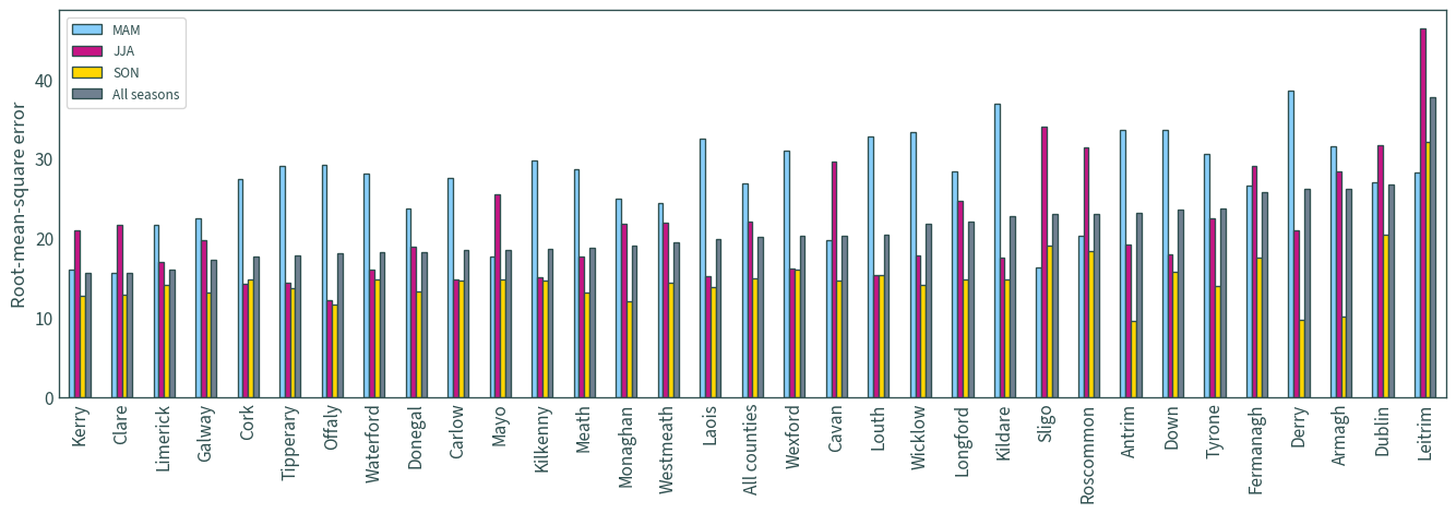
RMSE

rmse_all(df_p, mera_p)

	County	MAM	JJA	SON	All seasons
12	Kerry	16.088698	20.980745	12.831076	15.626586
4	Clare	15.620777	21.667300	12.927324	15.633088
17	Limerick	21.694449	17.040297	14.138739	16.041494
11	Galway	22.510660	19.779726	13.238386	17.312207
5	Cork	27.528523	14.363965	14.801772	17.706321
26	Tipperary	29.055517	14.384537	13.760518	17.939943
23	Offaly	29.297853	12.224616	11.762283	18.161581
28	Waterford	28.135305	16.148331	14.918000	18.246902
7	Donegal	23.725832	18.934147	13.284744	18.276909
2	Carlow	27.568439	14.852066	14.657607	18.500797
20	Mayo	17.791783	25.617337	14.876125	18.593063
14	Kilkenny	29.840210	15.086797	14.742384	18.743731
21	Meath	28.701678	17.733184	13.223505	18.904683
22	Monaghan	24.958436	21.906898	12.141298	19.051152
29	Westmeath	24.393357	21.923256	14.402558	19.473629
15	Laois	32.548061	15.311542	13.891385	19.869766
32	All counties	26.900422	22.151197	14.943157	20.244334
30	Wexford	31.020640	16.291702	16.074415	20.281861
3	Cavan	19.786513	29.673312	14.784902	20.312790
19	Louth	32.771328	15.443042	15.421298	20.524200
31	Wicklow	33.336165	17.941231	14.234892	21.837576
18	Longford	28.369177	24.749977	14.838420	22.114750
13	Kildare	36.875293	17.646973	14.913919	22.846667
25	Sligo	16.414317	34.052303	19.098170	23.114188
24	Roscommon	20.413333	31.472297	18.451814	23.153673
0	Antrim	33.686875	19.180885	9.665893	23.283869
8	Down	33.674826	17.986519	15.793475	23.699078
27	Tyrone	30.697184	22.485951	14.027558	23.805349
10	Fermanagh	26.660807	29.142878	17.607579	25.896450
6	Derry	38.610353	20.977881	9.811839	26.207623
1	Armagh	31.567006	28.379396	10.241772	26.282628
9	Dublin	27.058282	31.715537	20.425508	26.779954
16	Leitrim	28.285777	46.385272	32.191560	37.800448

rmse_all(df_p, mera_p).plot.bar(
    figsize=(14, 5),
    x="County",
    edgecolor="darkslategrey",
    color=["lightskyblue", "mediumvioletred", "gold", "slategrey"],
)
plt.xlabel("")
plt.ylabel("Root-mean-square error")
plt.tight_layout()
plt.show()

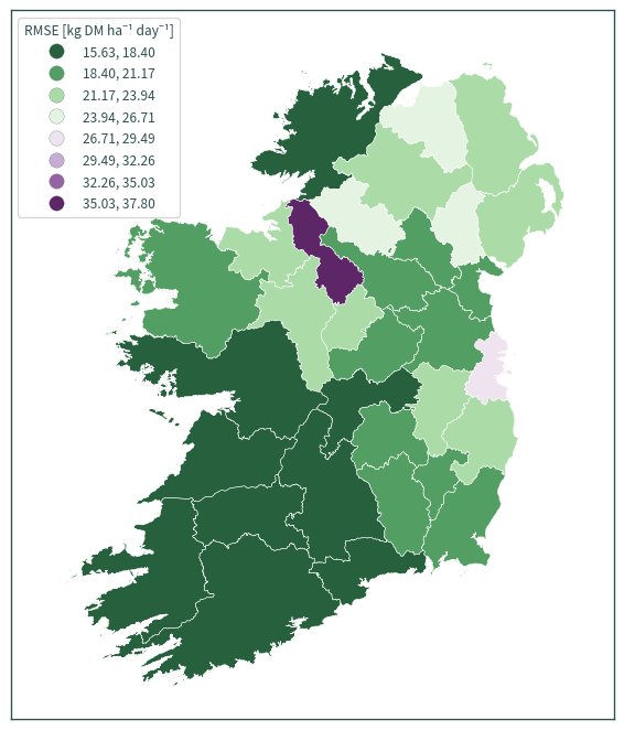
ie_counties = gpd.read_file(
    os.path.join("data", "boundaries", "boundaries_all.gpkg"),
    layer="OSi_OSNI_IE_Counties_2157",
)

ie_counties["COUNTY"] = ie_counties["COUNTY"].str.capitalize()

county_map = ie_counties.merge(
    rmse_all(df_p, mera_p), left_on="COUNTY", right_on="County"
)

ax = county_map.plot(
    column="All seasons",
    legend=True,
    cmap="PRGn_r",
    scheme="equal_interval",
    k=8,
    legend_kwds={
        "loc": "upper left",
        "fmt": "{:.2f}",
        "title": "RMSE [kg DM ha⁻¹ day⁻¹]",
    },
    figsize=(6, 7),
    alpha=0.85,
)
county_map.boundary.plot(ax=ax, color="white", linewidth=0.3)
# county_map.boundary.plot(ax=ax, color="darkslategrey", linewidth=0.3)
ax.tick_params(labelbottom=False, labelleft=False)
for legend_handle in ax.get_legend().legend_handles:
    legend_handle.set_markeredgewidth(0.2)
    legend_handle.set_markeredgecolor("darkslategrey")
plt.axis("equal")
plt.tight_layout()
plt.show()

Linear regression - all counties

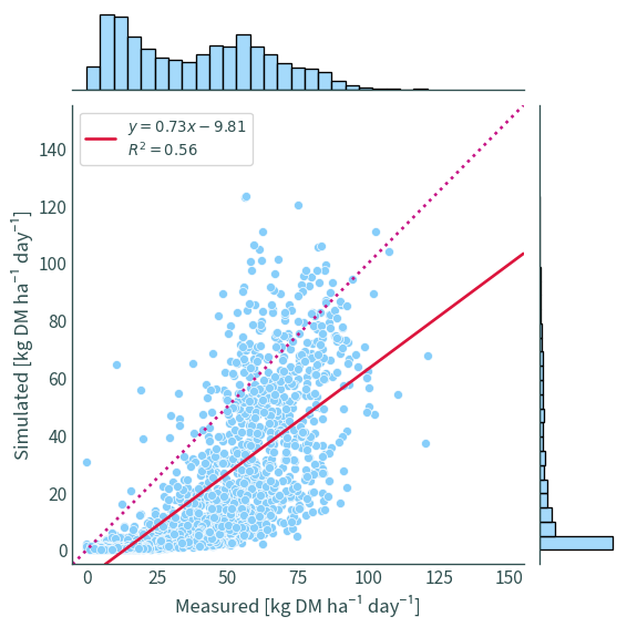
MAM

get_linear_regression(df_p, mera_p, county=None, season="MAM")

                            OLS Regression Results                            
==============================================================================
Dep. Variable:              Simulated   R-squared:                       0.559
Model:                            OLS   Adj. R-squared:                  0.558
Method:                 Least Squares   F-statistic:                     2590.
Date:                Fri, 01 Dec 2023   Prob (F-statistic):               0.00
Time:                        22:30:06   Log-Likelihood:                -8618.3
No. Observations:                2049   AIC:                         1.724e+04
Df Residuals:                    2047   BIC:                         1.725e+04
Df Model:                           1                                         
Covariance Type:            nonrobust                                         
==============================================================================
                 coef    std err          t      P>|t|      [0.025      0.975]
------------------------------------------------------------------------------
const         -9.8076      0.664    -14.765      0.000     -11.110      -8.505
Measured       0.7296      0.014     50.893      0.000       0.701       0.758
==============================================================================
Omnibus:                      453.979   Durbin-Watson:                   0.729
Prob(Omnibus):                  0.000   Jarque-Bera (JB):             1260.953
Skew:                           1.151   Prob(JB):                    1.54e-274
Kurtosis:                       6.077   Cond. No.                         85.8
==============================================================================

Notes:
[1] Standard Errors assume that the covariance matrix of the errors is correctly specified.

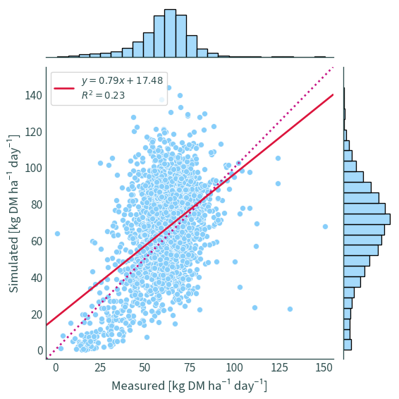
JJA

get_linear_regression(df_p, mera_p, county=None, season="JJA")

                            OLS Regression Results                            
==============================================================================
Dep. Variable:              Simulated   R-squared:                       0.232
Model:                            OLS   Adj. R-squared:                  0.231
Method:                 Least Squares   F-statistic:                     645.6
Date:                Fri, 01 Dec 2023   Prob (F-statistic):          1.09e-124
Time:                        22:30:08   Log-Likelihood:                -9602.7
No. Observations:                2142   AIC:                         1.921e+04
Df Residuals:                    2140   BIC:                         1.922e+04
Df Model:                           1                                         
Covariance Type:            nonrobust                                         
==============================================================================
                 coef    std err          t      P>|t|      [0.025      0.975]
------------------------------------------------------------------------------
const         17.4848      1.940      9.013      0.000      13.681      21.289
Measured       0.7894      0.031     25.408      0.000       0.728       0.850
==============================================================================
Omnibus:                       15.305   Durbin-Watson:                   0.852
Prob(Omnibus):                  0.000   Jarque-Bera (JB):               16.118
Skew:                           0.173   Prob(JB):                     0.000316
Kurtosis:                       3.248   Cond. No.                         262.
==============================================================================

Notes:
[1] Standard Errors assume that the covariance matrix of the errors is correctly specified.

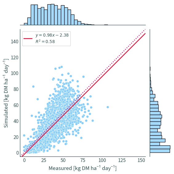
SON

get_linear_regression(df_p, mera_p, county=None, season="SON")

                            OLS Regression Results                            
==============================================================================
Dep. Variable:              Simulated   R-squared:                       0.584
Model:                            OLS   Adj. R-squared:                  0.583
Method:                 Least Squares   F-statistic:                     2727.
Date:                Fri, 01 Dec 2023   Prob (F-statistic):               0.00
Time:                        22:30:08   Log-Likelihood:                -7985.8
No. Observations:                1947   AIC:                         1.598e+04
Df Residuals:                    1945   BIC:                         1.599e+04
Df Model:                           1                                         
Covariance Type:            nonrobust                                         
==============================================================================
                 coef    std err          t      P>|t|      [0.025      0.975]
------------------------------------------------------------------------------
const         -2.3835      0.745     -3.198      0.001      -3.845      -0.922
Measured       0.9811      0.019     52.217      0.000       0.944       1.018
==============================================================================
Omnibus:                      225.214   Durbin-Watson:                   0.955
Prob(Omnibus):                  0.000   Jarque-Bera (JB):              377.170
Skew:                           0.787   Prob(JB):                     1.25e-82
Kurtosis:                       4.474   Cond. No.                         89.2
==============================================================================

Notes:
[1] Standard Errors assume that the covariance matrix of the errors is correctly specified.

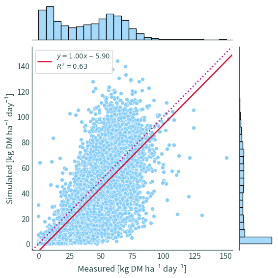
All seasons

get_linear_regression(df_p, mera_p, county=None)

                            OLS Regression Results                            
==============================================================================
Dep. Variable:              Simulated   R-squared:                       0.631
Model:                            OLS   Adj. R-squared:                  0.631
Method:                 Least Squares   F-statistic:                 1.266e+04
Date:                Fri, 01 Dec 2023   Prob (F-statistic):               0.00
Time:                        22:30:10   Log-Likelihood:                -32473.
No. Observations:                7414   AIC:                         6.495e+04
Df Residuals:                    7412   BIC:                         6.496e+04
Df Model:                           1                                         
Covariance Type:            nonrobust                                         
==============================================================================
                 coef    std err          t      P>|t|      [0.025      0.975]
------------------------------------------------------------------------------
const         -5.9006      0.410    -14.399      0.000      -6.704      -5.097
Measured       0.9959      0.009    112.534      0.000       0.979       1.013
==============================================================================
Omnibus:                      359.378   Durbin-Watson:                   0.622
Prob(Omnibus):                  0.000   Jarque-Bera (JB):              839.837
Skew:                           0.298   Prob(JB):                    4.28e-183
Kurtosis:                       4.538   Cond. No.                         84.6
==============================================================================

Notes:
[1] Standard Errors assume that the covariance matrix of the errors is correctly specified.

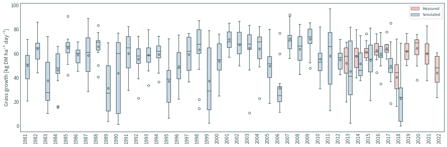
Box plots

def box_plots(counties, season):
    for county in counties:
        plot_data = data_all[(data_all["county"] == county)]
        # keep season data
        if season == "MAM":
            plot_data = plot_data[
                (plot_data.index.month == 3)
                | (plot_data.index.month == 4)
                | (plot_data.index.month == 5)
            ]
        elif season == "JJA":
            plot_data = plot_data[
                (plot_data.index.month == 6)
                | (plot_data.index.month == 7)
                | (plot_data.index.month == 8)
            ]
        fig, ax = plt.subplots(figsize=(15, 5))
        sns.boxplot(
            x=plot_data.index.year,
            y=plot_data["value"],
            hue=plot_data["data"],
            ax=ax,
            palette="Pastel1",
            showmeans=True,
            meanprops={
                "markeredgecolor": "darkslategrey",
                "marker": "d",
                "markerfacecolor": (1, 1, 0, 0),
                "markersize": 4.5,
            },
            flierprops={
                "marker": "o",
                "markerfacecolor": (1, 1, 0, 0),
                "markeredgecolor": "darkslategrey",
            },
            boxprops={"edgecolor": "darkslategrey", "alpha": 0.75},
            whiskerprops={"color": "darkslategrey", "alpha": 0.75},
            capprops={"color": "darkslategrey", "alpha": 0.75},
            medianprops={"color": "darkslategrey", "alpha": 0.75},
        )
        plt.xlabel("")
        ax.tick_params(axis="x", rotation=90)
        plt.ylabel("Grass growth [kg DM ha⁻¹ day⁻¹]")
        # plt.title(county)
        plt.legend(title=None)
        plt.tight_layout()
        print(county)
        plt.show()

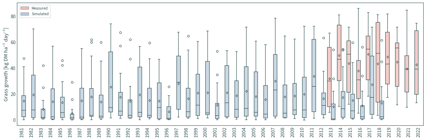
MAM growth grouped by year

box_plots(["Wexford"], "MAM")

Wexford

JJA growth grouped by year

box_plots(["Wexford"], "JJA")

Wexford