PastureBase Ireland

https://pasturebase.teagasc.ie

Hanrahan, L., Geoghegan, A., O’Donovan, M., Griffith, V., Ruelle, E., Wallace, M. and Shalloo, L. (2017). ‘PastureBase Ireland: A grassland decision support system and national database’, Computers and Electronics in Agriculture, vol. 136, pp. 193-201. DOI: 10.1016/j.compag.2017.01.029.

import os
from datetime import datetime, timezone
import matplotlib.colors as mcolors
import matplotlib.pyplot as plt
import numpy as np
import pandas as pd
from matplotlib.cbook import boxplot_stats

DATA_DIR = os.path.join(
    "data", "grass_growth", "PastureBaseIreland", "GrowthRateAveragebyWeek.csv"
)

grass = pd.read_csv(DATA_DIR)

grass.head()

	Name	Counties_CountyID	Year	WeekNo	AvgGrowth
0	Antrim	1	2019	37	NaN
1	Armagh	2	2018	22	126.17
2	Armagh	2	2018	23	93.01
3	Armagh	2	2018	24	25.58
4	Armagh	2	2018	25	35.34

grass.shape

(12455, 5)

list(grass)

['Name', 'Counties_CountyID', 'Year', 'WeekNo', 'AvgGrowth']

grass.sort_values(by=["Name", "Year", "WeekNo"], inplace=True)

# convert year and week number to timestamp
# (Monday as the first day of the week)
grass["Timestamp"] = grass.apply(
    lambda row: datetime.strptime(
        str(row.Year) + "-" + str(row.WeekNo) + "-1", "%G-%V-%u"
    ),
    axis=1,
)

# create time series using counties as individual columns
grass.drop(columns=["Counties_CountyID"], inplace=True)

grass.head()

	Name	Year	WeekNo	AvgGrowth	Timestamp
0	Antrim	2019	37	NaN	2019-09-09
1	Armagh	2018	22	126.17	2018-05-28
2	Armagh	2018	23	93.01	2018-06-04
3	Armagh	2018	24	25.58	2018-06-11
4	Armagh	2018	25	35.34	2018-06-18

grass_ts = pd.pivot_table(
    grass[["Name", "AvgGrowth", "Timestamp"]],
    values="AvgGrowth",
    index=["Timestamp"],
    columns=["Name"],
)

grass_ts.shape

(508, 30)

grass_ts["time"] = grass_ts.index

grass_ts.sort_values(by=["time"], inplace=True)

grass_ts.head()

Name	Armagh	Carlow	Cavan	Clare	Cork	Derry	Donegal	Down	Dublin	Galway	...	Offaly	Roscommon	Sligo	Tipperary	Tyrone	Waterford	Westmeath	Wexford	Wicklow	time
Timestamp
2012-12-31	NaN	NaN	0.39	NaN	1.10	NaN	NaN	NaN	NaN	1.71	...	NaN	NaN	NaN	17.05	NaN	NaN	NaN	NaN	3.36	2012-12-31
2013-01-07	NaN	NaN	4.33	4.94	4.97	NaN	NaN	NaN	NaN	0.00	...	NaN	NaN	NaN	3.66	NaN	8.76	NaN	NaN	NaN	2013-01-07
2013-01-14	NaN	NaN	NaN	NaN	4.46	NaN	NaN	NaN	NaN	7.14	...	NaN	NaN	NaN	5.43	NaN	3.22	NaN	3.47	NaN	2013-01-14
2013-01-21	NaN	NaN	NaN	2.42	10.11	NaN	NaN	NaN	NaN	0.00	...	NaN	NaN	3.45	5.00	NaN	3.89	NaN	6.02	NaN	2013-01-21
2013-01-28	NaN	5.03	4.80	NaN	7.67	NaN	NaN	NaN	NaN	6.87	...	NaN	NaN	NaN	5.11	NaN	4.64	NaN	NaN	3.37	2013-01-28

5 rows × 31 columns

# drop NI counties
grass_ts.drop(columns=["Armagh", "Derry", "Down", "Tyrone"], inplace=True)

# use weekly time series starting on Monday to fill missing rows
grass_ = pd.DataFrame(
    pd.date_range(
        str(grass_ts["time"][0].year) + "-01-01",
        str(grass_ts["time"][len(grass_ts) - 1].year) + "-12-31",
        freq="W-MON",
    ),
    columns=["time"],
)

grass_ts = pd.merge(grass_, grass_ts, how="outer")

grass_ts.index = grass_ts["time"]

grass_ts.drop(columns=["time"], inplace=True)

grass_ts.shape

(574, 26)

# new colour map
# https://stackoverflow.com/a/31052741
# sample the colormaps that you want to use. Use 15 from each so we get 30
# colors in total
colors1 = plt.cm.tab20b(np.linspace(0.0, 1, 15))
colors2 = plt.cm.tab20c(np.linspace(0, 1, 15))

# combine them and build a new colormap
colors = np.vstack((colors1, colors2))

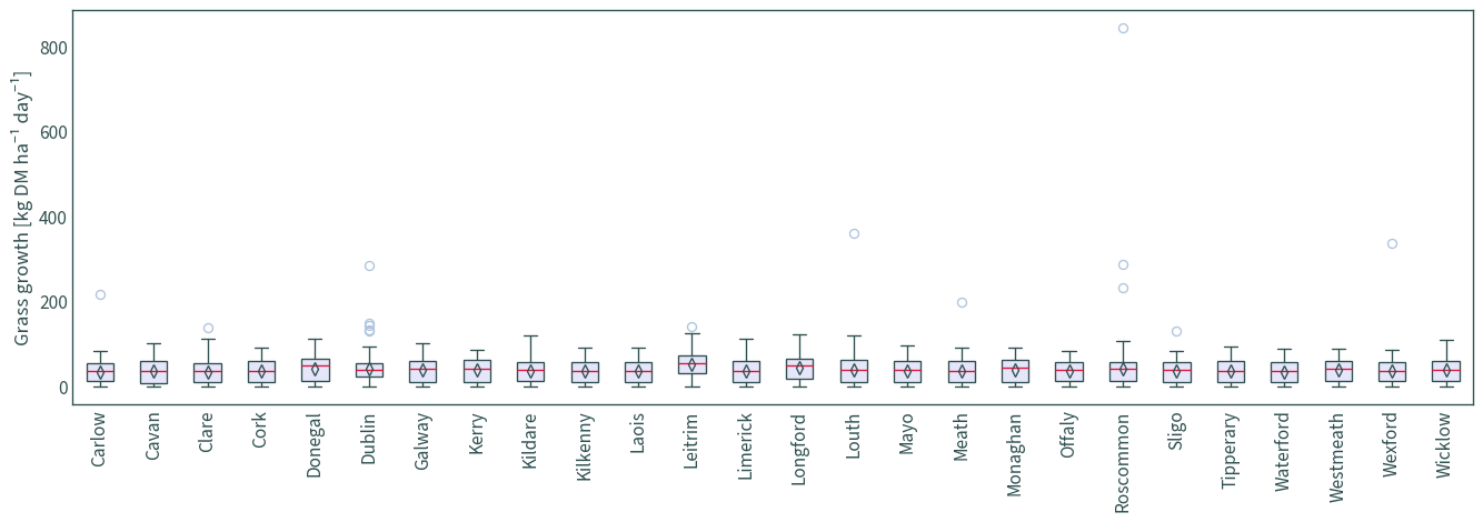
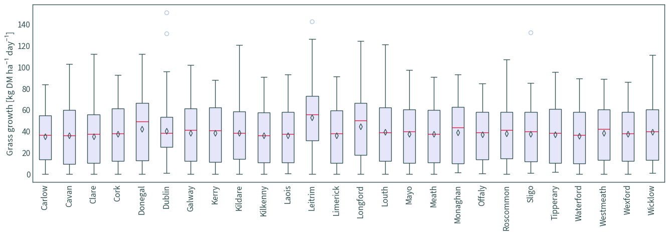
Distribution

# with outliers
grass_ts.plot.box(
    figsize=(14, 5),
    showmeans=True,
    patch_artist=True,
    color={
        "medians": "Crimson",
        "whiskers": "DarkSlateGrey",
        "caps": "DarkSlateGrey",
    },
    boxprops={"facecolor": "Lavender", "color": "DarkSlateGrey"},
    meanprops={
        "markeredgecolor": "DarkSlateGrey",
        "marker": "d",
        "markerfacecolor": (1, 1, 0, 0),  # transparent
    },
    flierprops={"markeredgecolor": "LightSteelBlue", "zorder": 1},
)
plt.xticks(rotation="vertical")
plt.ylabel("Grass growth [kg DM ha⁻¹ day⁻¹]")
plt.tight_layout()
plt.show()

Time series

counties = list(grass_ts)

# pivot table for plotting
grass_piv = grass_ts.copy()
grass_piv["year"] = grass_piv.index.year
grass_piv["weekno"] = grass_piv.index.isocalendar().week
grass_piv = pd.pivot_table(grass_piv, index="weekno", columns="year")

grass_piv.head()

	Carlow										...	Wicklow
year	2013	2014	2015	2016	2017	2018	2019	2020	2021	2022	...	2013	2014	2015	2016	2017	2018	2019	2020	2021	2022
weekno
1	NaN	4.90	NaN	NaN	3.56	5.16	4.635	NaN	NaN	6.08	...	4.28	NaN	NaN	NaN	NaN	7.35	5.71	NaN	NaN	NaN
2	NaN	NaN	NaN	NaN	NaN	8.25	7.830	NaN	NaN	10.04	...	NaN	NaN	NaN	NaN	NaN	NaN	5.98	5.16	5.10	14.06
3	NaN	NaN	NaN	7.57	2.97	3.98	8.610	NaN	3.25	1.46	...	NaN	4.35	6.68	5.57	NaN	4.24	5.40	5.96	4.17	10.44
4	NaN	NaN	NaN	5.14	2.16	20.05	9.300	3.76	13.59	4.76	...	NaN	4.02	3.81	3.35	NaN	2.68	6.53	6.15	5.00	8.25
5	5.03	4.11	3.80	NaN	NaN	4.31	8.650	3.33	3.16	4.62	...	3.37	NaN	NaN	NaN	NaN	4.37	10.75	4.90	6.14	5.18
6	NaN	NaN	3.50	0.74	4.35	5.20	8.790	5.64	3.68	3.82	...	3.84	0.96	3.44	5.42	7.36	6.37	25.03	9.46	4.14	4.50
7	NaN	NaN	2.07	0.00	10.19	3.64	6.720	3.44	2.63	8.25	...	NaN	NaN	1.79	6.96	NaN	3.72	10.06	6.52	2.39	17.63
8	14.40	7.73	3.16	NaN	9.76	6.31	7.080	5.35	6.38	7.63	...	3.73	2.79	3.42	4.86	11.18	6.08	7.52	10.33	10.72	21.14
9	7.15	NaN	3.51	5.83	12.97	1.94	14.630	7.19	6.16	7.87	...	NaN	8.06	8.65	4.22	8.43	9.51	21.20	4.88	7.94	7.81
10	8.59	6.20	12.36	6.49	17.16	4.30	19.380	9.12	14.76	9.46	...	5.68	5.09	4.03	4.73	11.08	3.76	17.01	8.99	8.68	42.61
11	11.53	11.54	9.34	9.59	14.15	1.55	14.520	12.69	10.99	8.97	...	NaN	14.98	8.45	7.08	15.42	6.10	11.28	10.82	14.48	15.93
12	10.62	14.92	13.48	12.94	29.57	9.46	28.140	16.59	15.91	14.58	...	5.52	14.55	14.38	10.81	16.58	2.53	19.24	12.42	15.99	13.94
13	10.11	17.97	18.43	12.89	29.32	8.41	22.920	17.22	27.74	18.71	...	12.27	18.58	21.43	12.87	26.09	8.80	33.88	14.18	26.31	16.97
14	6.74	27.54	16.96	218.31	36.72	11.69	25.220	22.36	37.10	34.00	...	1.08	32.47	34.09	14.05	33.87	5.23	27.36	22.52	29.04	36.60
15	10.96	28.29	32.26	30.21	38.20	20.44	25.210	39.46	42.83	32.96	...	8.33	40.62	36.10	19.90	47.85	18.23	36.87	36.49	40.04	34.63
16	14.96	38.19	39.05	33.17	50.56	44.45	33.400	52.13	35.67	36.63	...	13.20	47.64	47.23	29.14	50.08	39.89	40.20	53.25	37.35	35.74
17	32.35	43.56	59.42	36.16	54.78	61.83	55.400	65.82	47.20	48.64	...	38.81	54.80	59.28	34.73	51.24	55.63	106.52	67.52	45.58	50.23
18	42.62	50.26	44.75	39.94	48.45	55.51	69.290	61.86	49.68	56.26	...	39.65	65.05	45.02	36.08	67.15	53.05	64.63	63.56	50.15	50.43
19	48.45	48.46	44.17	44.28	57.79	62.89	57.930	61.98	62.51	62.62	...	35.54	84.47	58.63	43.71	58.14	72.66	63.59	65.18	46.50	60.57
20	46.13	59.81	61.64	74.84	58.34	66.17	60.420	59.36	57.76	80.15	...	61.61	65.31	61.08	89.75	71.77	68.18	64.97	57.51	57.16	76.91
21	51.25	59.40	58.83	83.00	77.29	83.54	67.490	47.78	70.53	77.27	...	78.20	60.46	57.86	83.51	96.39	83.48	70.16	54.04	69.57	80.65
22	44.28	75.11	63.11	68.60	81.22	71.60	69.960	73.73	71.14	63.51	...	56.92	49.72	76.47	79.02	92.53	91.16	84.70	61.46	65.88	70.36
23	58.14	59.43	59.93	78.92	67.68	70.16	73.260	36.77	81.54	60.29	...	71.38	69.57	74.09	71.89	74.25	77.26	80.82	48.18	86.88	57.00
24	50.47	70.67	63.39	57.46	66.53	44.06	59.670	35.36	79.01	64.98	...	56.52	54.21	57.60	71.98	75.83	56.10	62.89	39.23	85.19	62.55
25	49.41	73.66	62.46	64.87	62.64	36.11	54.830	41.15	67.93	58.89	...	62.08	72.68	66.20	53.15	75.28	48.92	73.57	56.07	68.17	59.93
26	60.67	53.59	54.06	63.79	56.68	29.13	65.170	58.01	45.44	46.49	...	55.04	62.66	53.91	75.10	62.11	33.44	75.70	78.29	52.01	63.43
27	38.29	47.75	43.12	66.39	62.96	17.66	65.950	77.71	54.64	49.26	...	61.21	47.00	55.41	61.57	71.23	19.74	70.78	83.08	56.54	54.78
28	54.03	44.82	52.23	68.11	69.82	14.75	44.810	69.82	52.93	58.28	...	39.23	55.18	54.75	66.11	78.86	15.69	60.52	64.27	55.04	62.77
29	20.31	44.90	59.74	51.68	51.38	20.47	36.970	72.50	57.67	58.66	...	44.67	67.60	61.96	61.10	65.03	11.87	63.53	71.83	67.18	56.59
30	9.67	52.36	59.55	70.17	72.64	10.98	40.150	64.57	47.26	41.46	...	25.12	47.22	68.05	66.04	57.99	4.40	66.09	71.54	59.48	49.45
31	19.44	40.31	57.15	43.76	65.00	30.51	50.670	63.57	26.17	33.38	...	43.17	47.32	59.80	61.73	71.00	39.34	68.23	72.17	37.04	38.11
32	62.28	22.45	66.82	47.53	58.08	36.32	46.220	61.88	43.79	39.57	...	59.95	46.48	64.16	68.49	70.72	111.08	62.22	66.32	50.71	46.33
33	71.13	41.93	53.34	42.01	63.32	46.17	53.280	66.97	53.48	35.20	...	52.84	46.98	64.26	55.55	74.44	67.16	64.06	64.56	65.03	37.65
34	48.44	52.50	54.56	29.55	61.95	35.14	59.410	60.48	70.76	28.66	...	48.64	58.53	53.51	62.42	64.57	78.54	61.79	68.90	68.87	33.92
35	40.49	45.48	57.85	42.76	70.09	61.68	61.340	54.74	54.61	28.41	...	48.42	43.26	55.34	58.97	61.58	57.67	71.89	61.88	71.87	35.51
36	15.02	49.39	55.69	55.31	65.25	42.19	54.610	58.14	48.64	32.85	...	37.04	50.43	61.16	60.15	64.01	58.08	71.94	53.17	61.30	30.43
37	18.82	51.07	48.06	55.17	61.79	52.10	50.880	57.57	46.64	32.36	...	45.70	45.97	52.02	59.47	50.70	61.65	54.65	51.26	53.13	33.95
38	17.89	49.14	45.24	52.05	48.04	51.04	47.530	59.82	44.88	47.58	...	17.58	45.88	59.29	60.46	45.39	59.28	64.68	61.72	57.16	43.11
39	23.76	37.84	47.11	59.79	61.75	51.72	43.210	51.92	47.82	NaN	...	57.35	54.63	41.45	49.56	48.52	47.86	60.04	53.57	51.42	NaN
40	23.28	42.90	49.60	50.44	40.26	41.00	47.270	36.57	41.13	NaN	...	37.87	51.51	41.28	58.69	39.62	38.69	50.57	47.40	50.79	NaN
41	43.42	38.52	40.77	41.97	37.17	41.55	45.120	49.81	37.41	NaN	...	35.02	37.44	36.68	42.23	35.30	35.61	53.49	34.42	45.18	NaN
42	40.67	32.17	38.15	41.27	40.00	36.73	28.400	24.79	31.92	NaN	...	36.82	31.21	30.96	27.88	30.01	44.45	41.73	31.74	38.20	NaN
43	33.25	32.67	30.21	33.88	29.95	29.21	21.910	27.05	31.78	NaN	...	31.52	28.92	28.87	32.14	23.62	30.62	33.51	26.87	34.16	NaN
44	24.23	24.39	29.56	26.44	23.32	23.18	25.600	18.57	31.23	NaN	...	27.22	27.54	23.21	29.94	20.23	27.99	13.39	19.68	26.38	NaN
45	26.06	22.42	19.91	25.25	20.21	17.13	13.040	16.72	21.85	NaN	...	30.18	11.47	27.23	5.06	21.34	25.38	17.91	19.82	32.09	NaN
46	14.26	16.66	21.85	17.62	25.93	22.43	13.390	18.63	15.61	NaN	...	12.63	38.28	17.30	NaN	21.11	32.38	21.19	12.71	19.15	NaN
47	16.43	7.27	12.43	13.43	NaN	15.97	10.320	17.12	14.64	NaN	...	9.16	NaN	16.66	10.72	NaN	3.67	5.61	11.34	17.78	NaN
48	8.93	NaN	1.87	14.17	29.64	17.77	5.580	8.04	15.79	NaN	...	NaN	6.17	9.19	NaN	5.76	8.63	4.87	12.65	15.32	NaN
49	6.09	8.15	12.22	12.76	9.05	8.49	10.530	15.74	11.15	NaN	...	3.25	13.04	NaN	8.85	8.01	NaN	4.84	8.66	9.60	NaN
50	NaN	NaN	6.61	NaN	NaN	10.12	6.880	5.08	9.23	NaN	...	NaN	NaN	NaN	NaN	NaN	NaN	7.76	9.62	NaN	NaN
51	NaN	NaN	14.11	4.13	8.24	NaN	5.760	NaN	4.71	NaN	...	NaN	NaN	NaN	10.89	NaN	NaN	6.10	NaN	5.71	NaN
52	NaN	NaN	NaN	NaN	NaN	NaN	NaN	7.83	8.81	NaN	...	NaN	NaN	NaN	NaN	NaN	NaN	NaN	NaN	8.00	NaN
53	NaN	NaN	8.09	NaN	NaN	NaN	NaN	5.39	NaN	NaN	...	NaN	NaN	NaN	NaN	NaN	NaN	NaN	NaN	NaN	NaN

53 rows × 271 columns

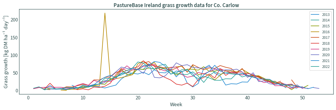
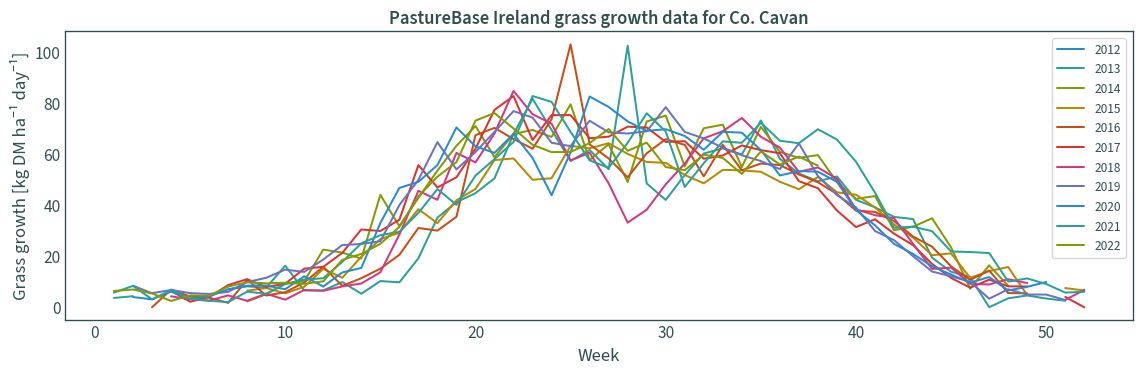
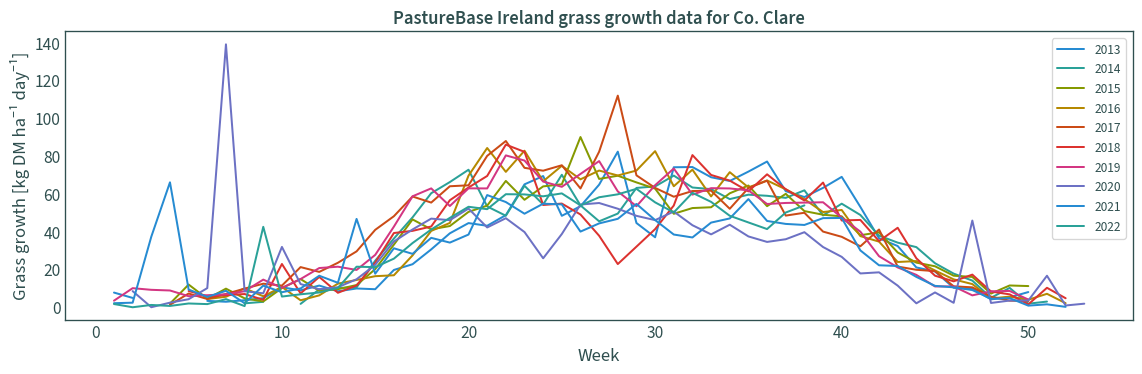
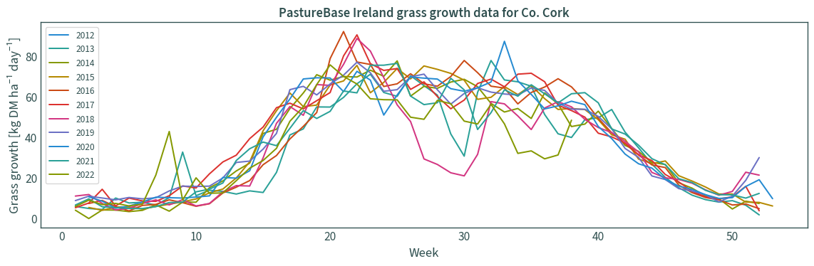
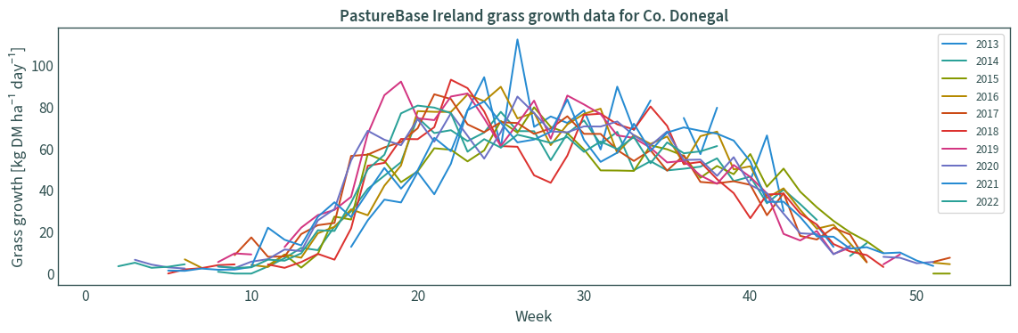
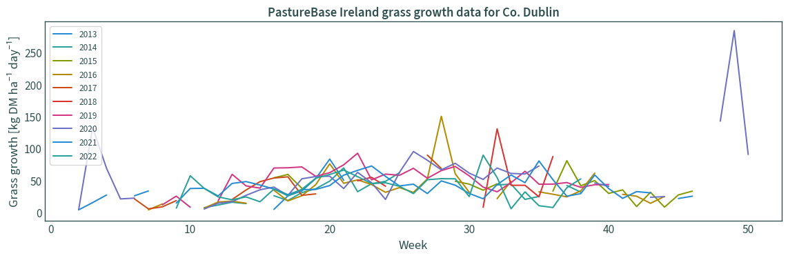
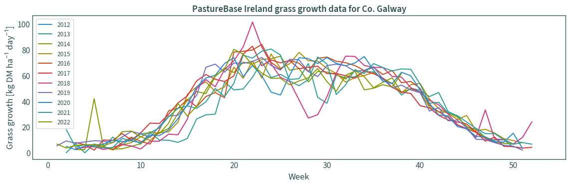
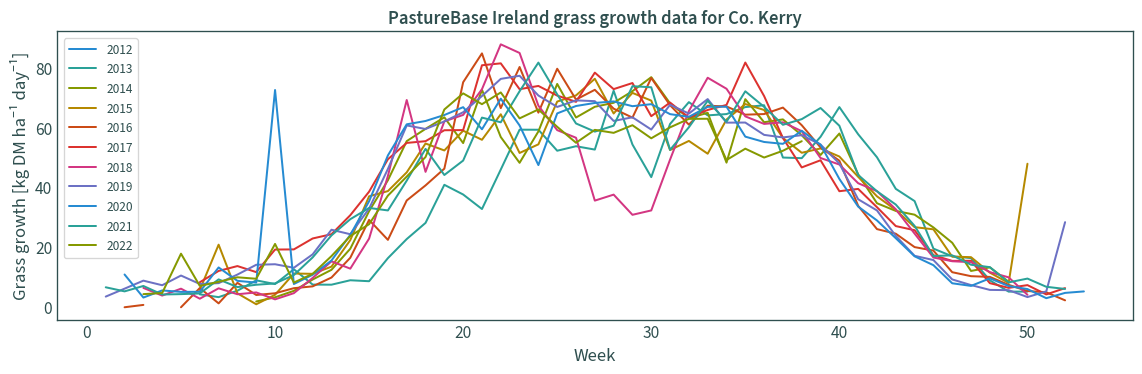
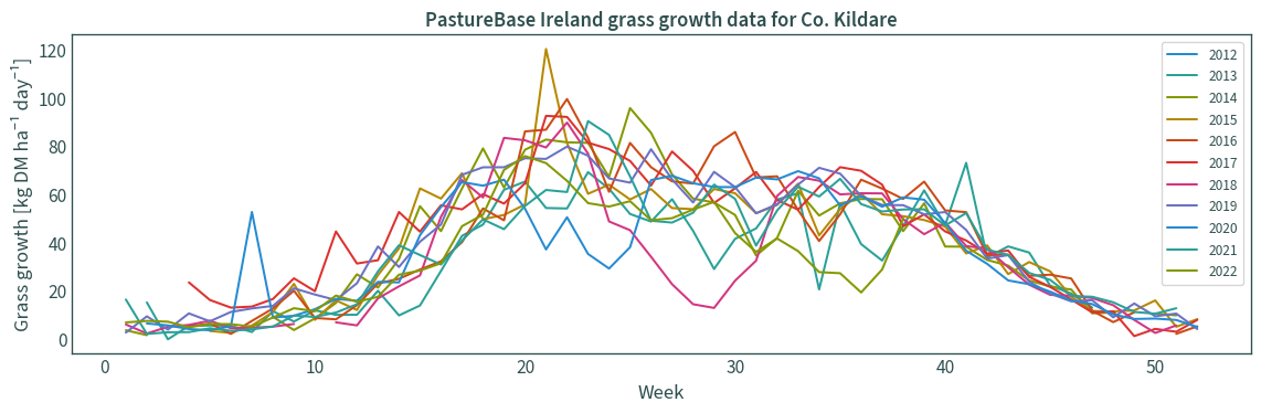
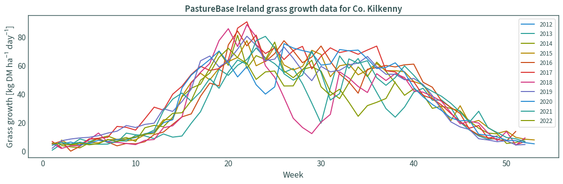
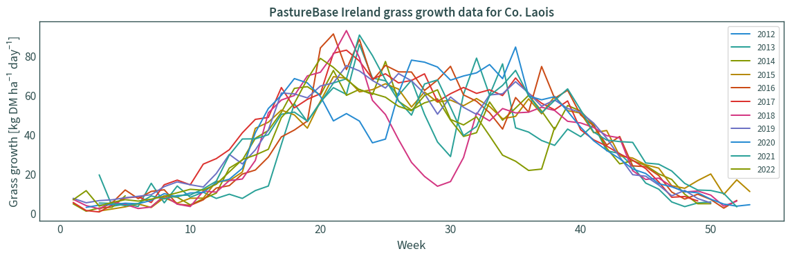
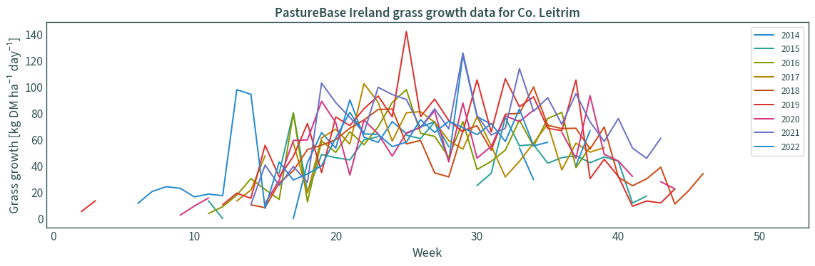
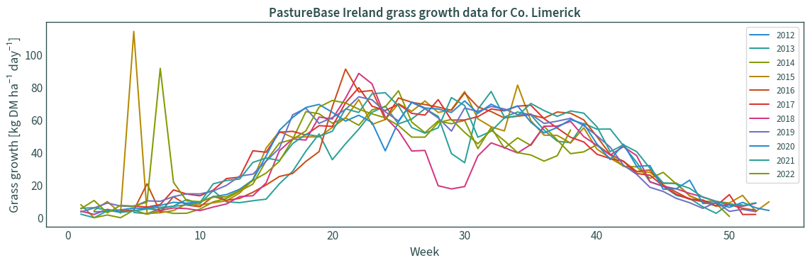
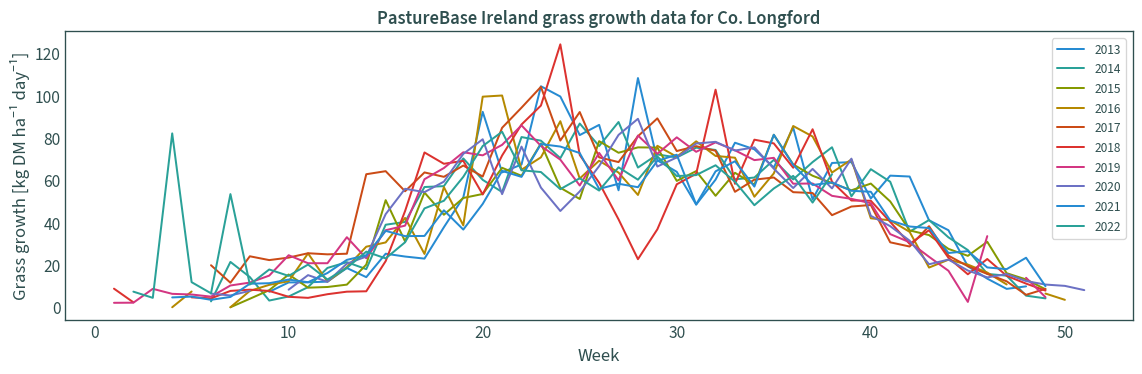
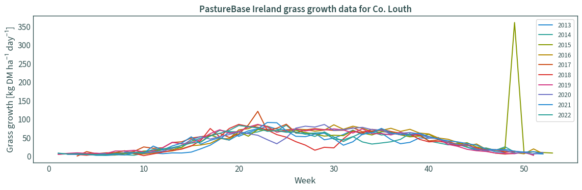
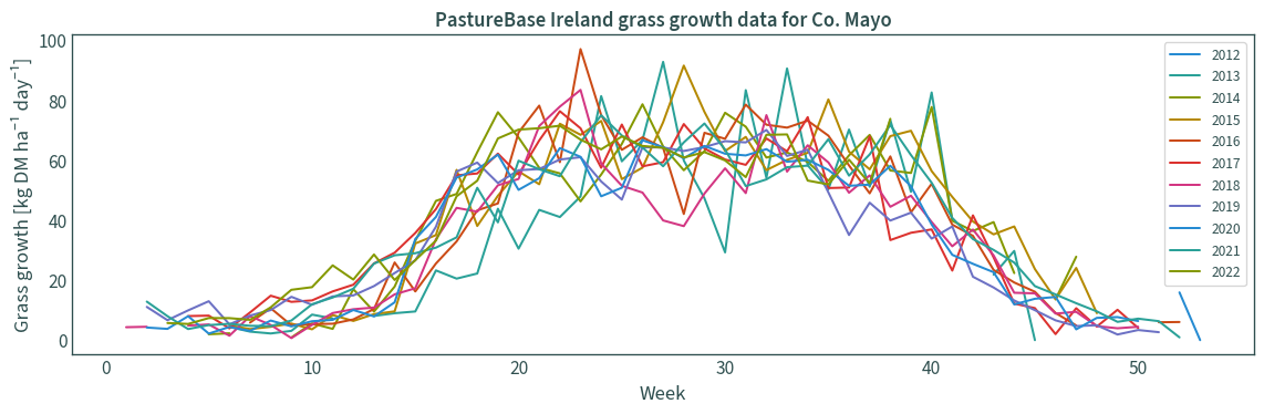
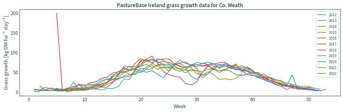
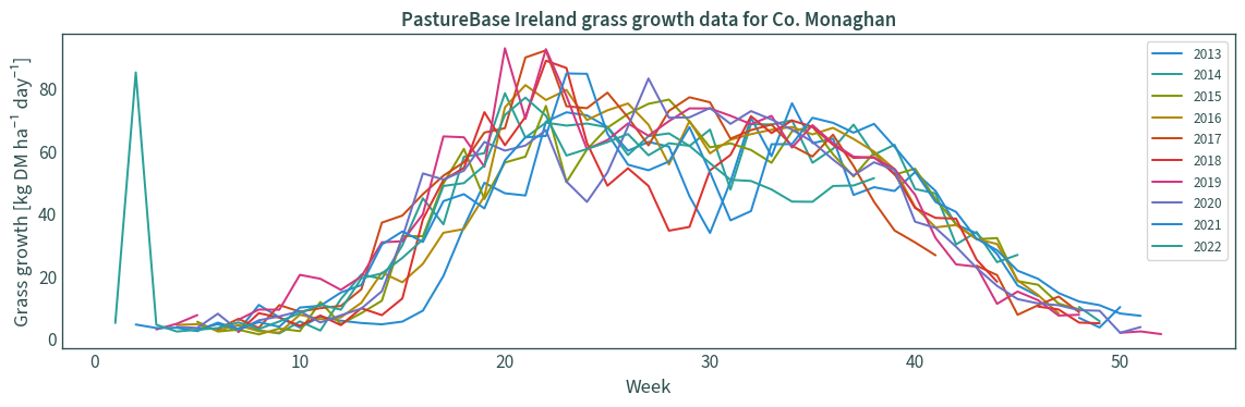
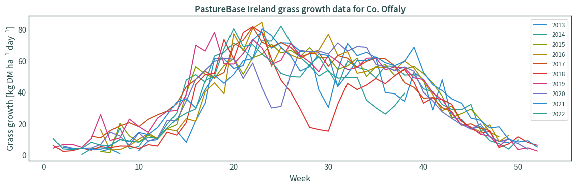
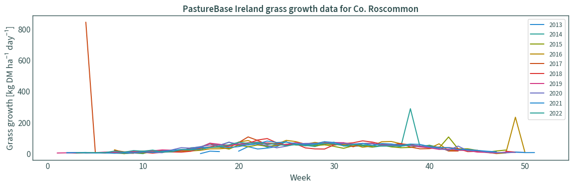
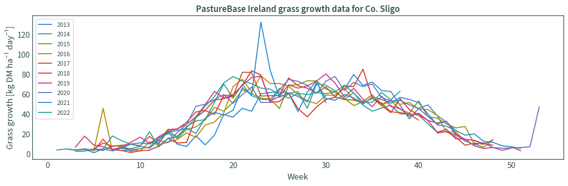
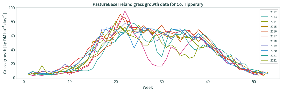
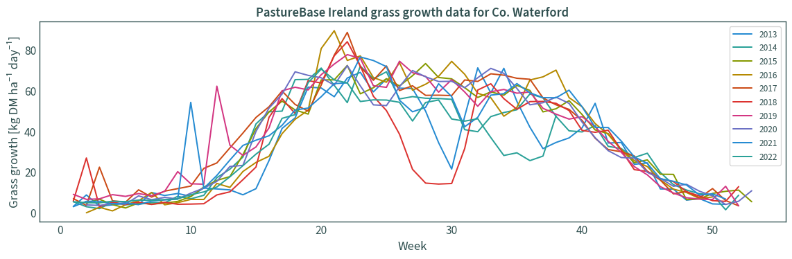
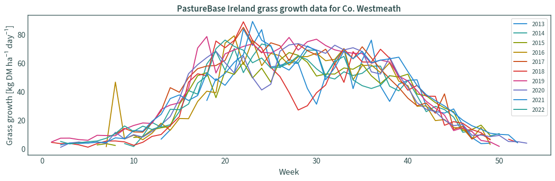
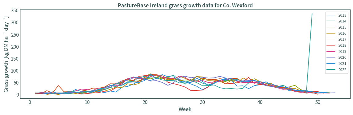
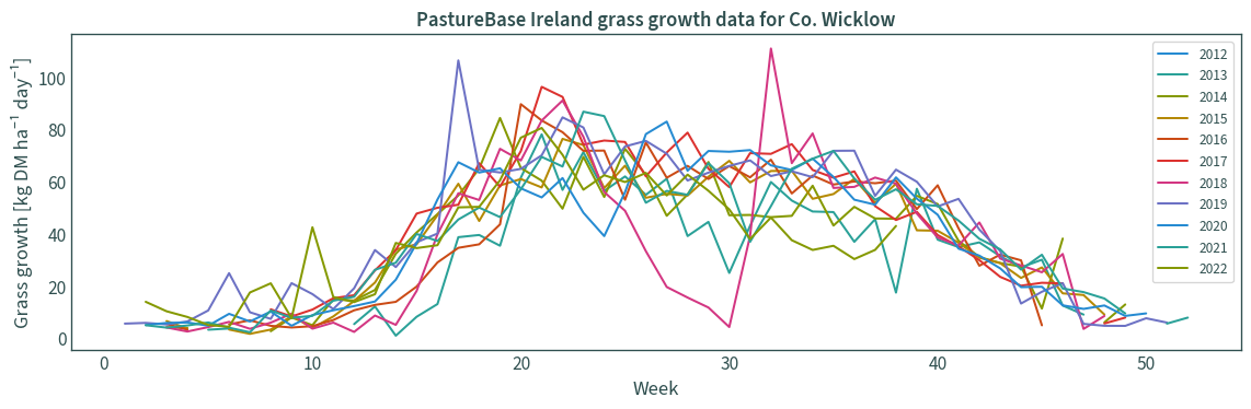
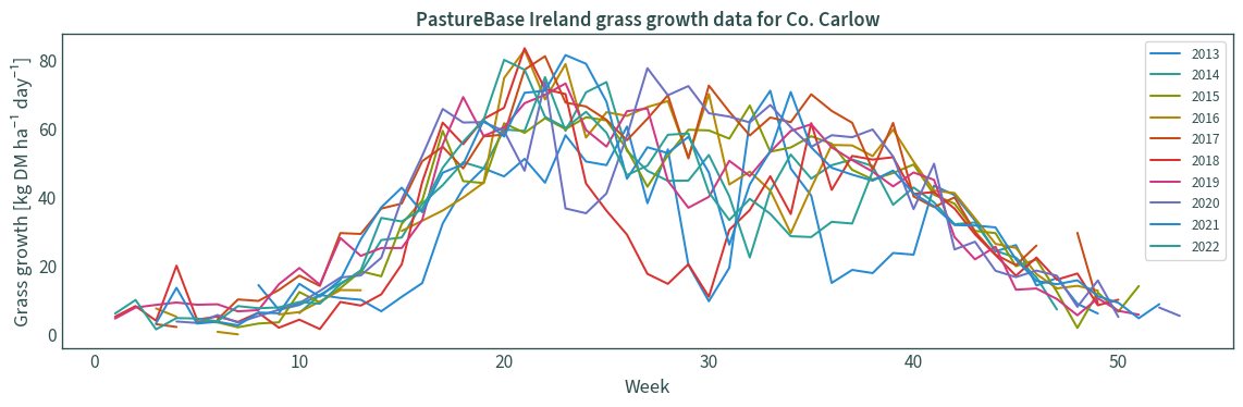
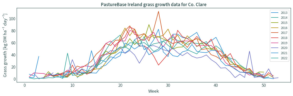
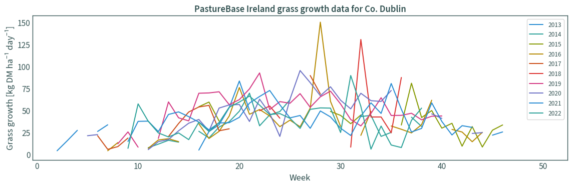
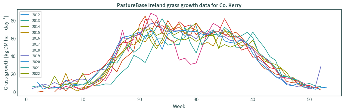
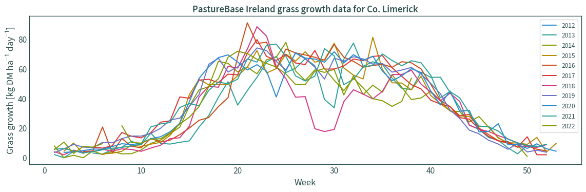
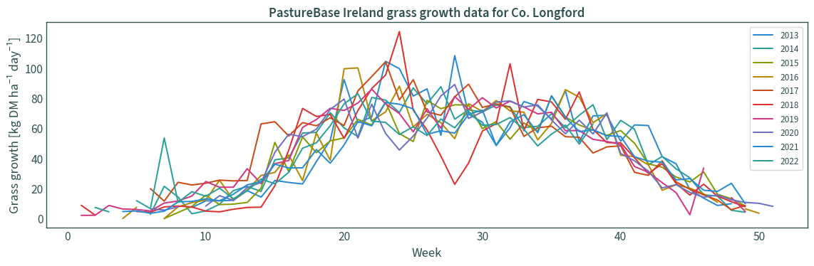
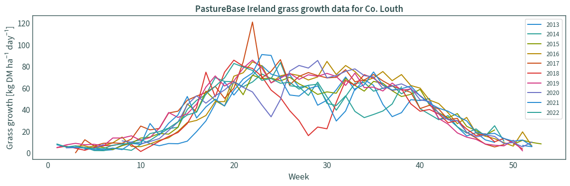
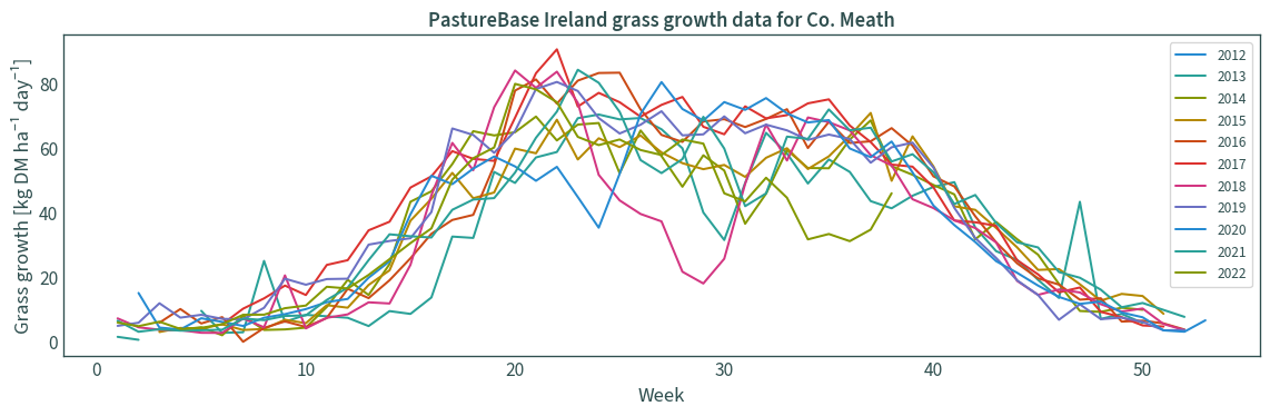
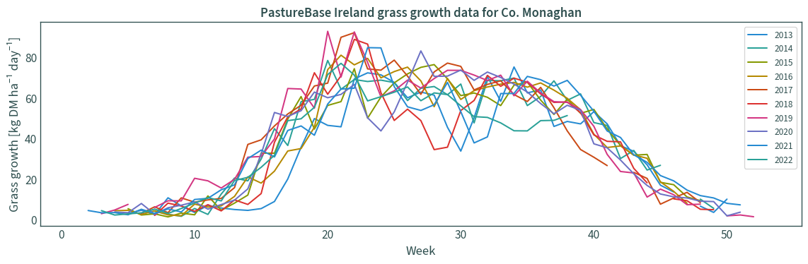
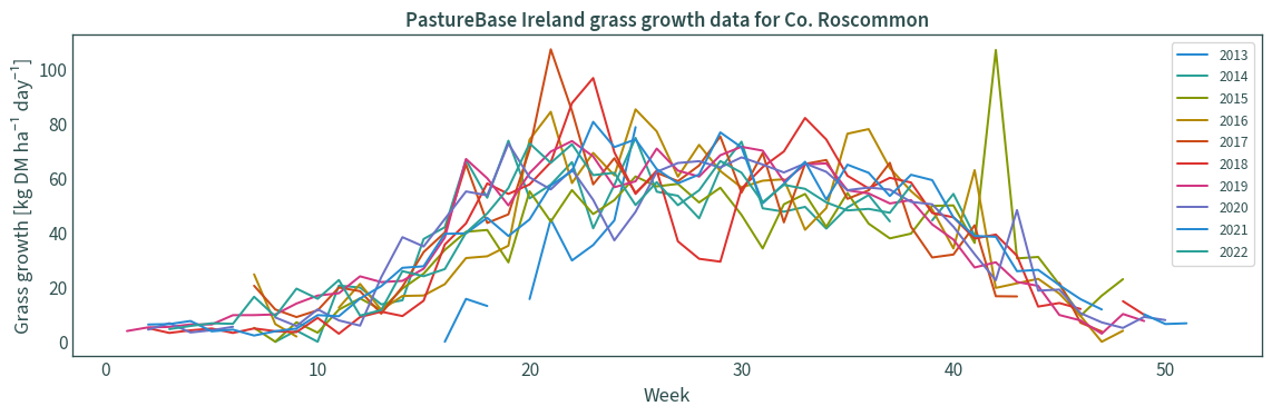
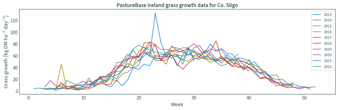
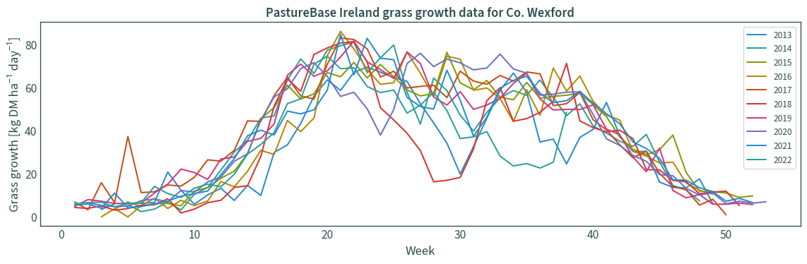
for county in counties:
    grass_piv[county].plot(
        figsize=(12, 4),
        xlabel="Week",
        ylabel="Grass growth [kg DM ha⁻¹ day⁻¹]",
    )
    plt.title(f"PastureBase Ireland grass growth data for Co. {county}")
    plt.legend(title=None)
    plt.tight_layout()
    plt.show()

Filtering outliers in distribution

grass_filter = grass_ts.melt(ignore_index=False)

grass_filter["weekno"] = grass_filter.index.isocalendar().week

grass_filter

	variable	value	weekno
time
2012-01-02	Carlow	NaN	1
2012-01-09	Carlow	NaN	2
2012-01-16	Carlow	NaN	3
2012-01-23	Carlow	NaN	4
2012-01-30	Carlow	NaN	5
...	...	...	...
2022-11-28	Wicklow	NaN	48
2022-12-05	Wicklow	NaN	49
2022-12-12	Wicklow	NaN	50
2022-12-19	Wicklow	NaN	51
2022-12-26	Wicklow	NaN	52

14924 rows × 3 columns

# filter all values over 180
grass_filter["value"] = np.where(
    grass_filter["value"] < 180, grass_filter["value"], np.nan
)

# filter all values over 60 when the week number is below 11
grass_filter["value"] = np.where(
    (grass_filter["weekno"] < 11) & (grass_filter["value"] > 60),
    np.nan,
    grass_filter["value"],
)

# filter all values over 40 when the week value is over 47
grass_filter["value"] = np.where(
    (grass_filter["weekno"] > 47) & (grass_filter["value"] > 40),
    np.nan,
    grass_filter["value"],
)

grass_filter

	variable	value	weekno
time
2012-01-02	Carlow	NaN	1
2012-01-09	Carlow	NaN	2
2012-01-16	Carlow	NaN	3
2012-01-23	Carlow	NaN	4
2012-01-30	Carlow	NaN	5
...	...	...	...
2022-11-28	Wicklow	NaN	48
2022-12-05	Wicklow	NaN	49
2022-12-12	Wicklow	NaN	50
2022-12-19	Wicklow	NaN	51
2022-12-26	Wicklow	NaN	52

14924 rows × 3 columns

# pivot table for plotting
grass_piv = pd.pivot_table(
    grass_filter[["variable", "value"]].reset_index(),
    values="value",
    index=["time"],
    columns=["variable"],
)
grass_piv["year"] = grass_piv.index.year
grass_piv["weekno"] = grass_piv.index.isocalendar().week
grass_piv = pd.pivot_table(grass_piv, index="weekno", columns="year")

grass_piv.tail()

variable	Carlow										...	Wicklow
year	2013	2014	2015	2016	2017	2018	2019	2020	2021	2022	...	2013	2014	2015	2016	2017	2018	2019	2020	2021	2022
weekno
49	6.09	8.15	12.22	12.76	9.05	8.49	10.53	15.74	11.15	NaN	...	3.25	13.04	NaN	8.85	8.01	NaN	4.84	8.66	9.60	NaN
50	NaN	NaN	6.61	NaN	NaN	10.12	6.88	5.08	9.23	NaN	...	NaN	NaN	NaN	NaN	NaN	NaN	7.76	9.62	NaN	NaN
51	NaN	NaN	14.11	4.13	8.24	NaN	5.76	NaN	4.71	NaN	...	NaN	NaN	NaN	10.89	NaN	NaN	6.10	NaN	5.71	NaN
52	NaN	NaN	NaN	NaN	NaN	NaN	NaN	7.83	8.81	NaN	...	NaN	NaN	NaN	NaN	NaN	NaN	NaN	NaN	8.00	NaN
53	NaN	NaN	8.09	NaN	NaN	NaN	NaN	5.39	NaN	NaN	...	NaN	NaN	NaN	NaN	NaN	NaN	NaN	NaN	NaN	NaN

5 rows × 271 columns

for county in counties:
    grass_piv[county].plot(
        figsize=(12, 4),
        xlabel="Week",
        ylabel="Grass growth [kg DM ha⁻¹ day⁻¹]",
    )
    plt.title(f"PastureBase Ireland grass growth data for Co. {county}")
    plt.legend(title=None)
    plt.tight_layout()
    plt.show()

# with outliers
grass_piv = pd.pivot_table(
    grass_filter[["variable", "value"]].reset_index(),
    values="value",
    index=["time"],
    columns=["variable"],
)
grass_piv.plot.box(
    figsize=(14, 5),
    showmeans=True,
    patch_artist=True,
    color={
        "medians": "Crimson",
        "whiskers": "DarkSlateGrey",
        "caps": "DarkSlateGrey",
    },
    boxprops={"facecolor": "Lavender", "color": "DarkSlateGrey"},
    meanprops={
        "markeredgecolor": "DarkSlateGrey",
        "marker": "d",
        "markerfacecolor": (1, 1, 0, 0),  # transparent
    },
    flierprops={"markeredgecolor": "LightSteelBlue", "zorder": 1},
)
plt.xticks(rotation="vertical")
plt.ylabel("Grass growth [kg DM ha⁻¹ day⁻¹]")
plt.tight_layout()
plt.show()

grass_filter = grass_filter.rename(columns={"variable": "county"})
grass_filter.to_csv(
    os.path.join(
        "data", "grass_growth", "PastureBaseIreland", "pasturebase_cleaned.csv"
    )
)

### Using boxplot stats

# grass_out = grass_ts.copy()
# for col in counties:
#     grass_out[[col]] = grass_out[[col]].replace(
#         list(boxplot_stats(grass_out[[col]].dropna())[0]["fliers"]), np.nan
#     )

# grass_out.plot.box(
#     figsize=(14, 5), showmeans=True, patch_artist=True,
#     color={
#         "medians": "Crimson",
#         "whiskers": "DarkSlateGrey",
#         "caps": "DarkSlateGrey"
#     },
#     boxprops={"facecolor": "Lavender", "color": "DarkSlateGrey"},
#     meanprops={
#         "markeredgecolor": "DarkSlateGrey",
#         "marker": "d",
#         "markerfacecolor": (1, 1, 0, 0)  # transparent
#     },
#     flierprops={"markeredgecolor": "LightSteelBlue", "zorder": 1}
# )
# plt.xticks(rotation="vertical")
# plt.ylabel("Grass growth [kg DM ha⁻¹ day⁻¹]")
# plt.tight_layout()
# plt.show()

# grass_out.diff().hist(figsize=(15, 18), bins=50, grid=False)
# plt.tight_layout()
# plt.show()

### Filtering outliers using 3-week moving average

# grass_out = grass_ts.reset_index()

# for county in counties:
#     mn = grass_out.rolling(3, center=True, on="time")[county].median()
#     # mn = grass_out.rolling(3, center=True, on="time")[county].mean()
#     # sd = grass_out.rolling(3, center=True, on="time")[county].std()
#     grass_out[f"{county}_outlier"] = (
#         grass_out[county].sub(mn).abs().gt(25)
#     )
#     grass_out[f"{county}_mn"] = mn
#     # grass_out[f"{county}_sd"] = sd
#     # grass_out[f"{county}_f"] = np.nan
#     # grass_out[f"{county}_f"] = grass_out[
#     #     (
#     #         grass_out[county] <=
#     #         grass_out[f"{county}_mn"] + 2 * grass_out[f"{county}_sd"]
#     #     ) & (
#     #         grass_out[county] >=
#     #         grass_out[f"{county}_mn"] - 2 * grass_out[f"{county}_sd"]
#     #     )
#     # ][[county]]
#     # grass_out[f"{county}_f"] = grass_out[
#     #     grass_out[f"{county}_f"].isna()
#     # ][[county]]

# grass_out.set_index("time", inplace=True)

# for county in counties:
#     axs = grass_out.plot(
#         # ylim=[0.0, 200.0],
#         figsize=(10, 4), y=county, label="growth"
#     )
#     grass_out.plot(
#         figsize=(10, 4), y=f"{county}_mn", ax=axs, label="moving_avg",
#         color="orange", zorder=1
#     )
#     # grass_out.plot(
#     #     figsize=(10, 4), y=f"{county}_f", ax=axs, label="f",
#     #     color="purple", linewidth=0.0, marker="*"
#     # )
#     if True in list(grass_out[f"{county}_outlier"].unique()):
#         grass_out[grass_out[f"{county}_outlier"] == True].plot(
#             ax=axs, linewidth=0.0, marker="*", y=county, label="outlier",
#             color="crimson"
#         )
#     plt.title(f"PastureBase Ireland grass growth data for Co. {county}")
#     plt.xlabel("")
#     plt.tight_layout()
#     plt.show()

# for county in counties:
#     axs = grass_out.plot(
#         # ylim=[0.0, 200.0],
#         figsize=(10, 4), y=county, label="growth"
#     )
#     grass_out.plot(
#         figsize=(10, 4), y=f"{county}_mn", ax=axs, label="moving_avg",
#         color="orange", zorder=1
#     )
#     if True in list(grass_out[f"{county}_outlier"].unique()):
#         grass_out[grass_out[f"{county}_outlier"] == True].plot(
#             ax=axs, linewidth=0.0, marker="*", y=county, label="outlier",
#             color="crimson"
#         )
#     plt.title(f"PastureBase Ireland grass growth data for Co. {county}")
#     plt.xlabel("")
#     plt.tight_layout()
#     plt.show()

# for county in counties:
#     axs = grass_out.loc["2017":"2019"].plot(
#         ylim=[0.0, 150.0],
#         figsize=(12, 8), y=county, label="growth"
#     )
#     grass_out.loc["2017":"2019"].plot(
#         figsize=(10, 4), y=f"{county}_mn", ax=axs, label="moving_avg",
#         color="orange", zorder=1
#     )
#     if True in list(
#         grass_out[f"{county}_outlier"].loc["2017":"2019"].unique()
#     ):
#         grass_out[
#             grass_out[f"{county}_outlier"] == True
#         ].loc["2017":"2019"].plot(
#             ax=axs, linewidth=0.0, marker="*", y=county, label="outlier",
#             color="crimson"
#         )
#     plt.title(f"PastureBase Ireland grass growth data for Co. {county}")
#     plt.xlabel("")
#     plt.tight_layout()
#     plt.show()